Foreword
Real estate vs stocks, the perennial debate. Which one should you invest in?
As usual, a reminder that I am not a financial professional by training — I am a software engineer by training, and by trade. The following is based on my personal understanding, which is gained through self-study and working in finance for a few years.
If you find anything that you feel is incorrect, please feel free to leave a comment, and discuss your thoughts.
Caveats
Before we go deeper into the discussion, I’d like to address some criticisms of “Monte Carlo“. To be absolutely clear, in “Monte Carlo” and in this post, I use simplified models to represent returns from various assets. In particular, stock returns have been modeled as normal distributions, which isn’t quite correct:

Right: Normal distribution with 12.2% mean returns and 19.7% standard deviation.
As you can see from the histograms, actual stock markets total returns (left) is quite different from the stylized normal distribution with similar mean and standard deviation.
Separately, assumptions that stocks and bonds (and in this post, real estate) returns are completely uncorrelated are clearly too permissive. In reality, stocks, bonds and real estate are somewhat (negatively) correlated over short periods of time, as all of them are generally affected by politics, inflation and interest rates, amongst other things.
That said, the point of “Monte Carlo” and this post isn’t to build a perfect model for anyone’s financial planning purposes. Instead, these 2 posts are meant to explore various aspects of portfolio construction — how you should think about expected returns, CAGR, SWR, and how volatility affects these metrics. With this rather more modest goal, I believe the simplified models used are more than adequate.
My my, what low returns you have!
In “My Personal Portfolio“, I mentioned that I invest heavily in real estate, generally via private real estate syndications.
In some private discussions about real estate syndications, others have noted that the pro forma returns presented by some real estate syndications that I invest with (generally in the 10-15% range) are lower than what the stock markets have returned in the past 20 years or so.
If you pick up a calculator, you’ll find that from 2009 – 2020 stocks have returned about 15.5% on average every year, with a CAGR of about 15%. Compared to the 10-15% pro forma returns, it seems silly to even consider real estate.
Therefore, we should just invest 100% in stocks… right?
Expected returns
The first problem with the 100% stocks assertion, is that expected returns are misleading — expected returns are merely “expected” as opposed to “realized”. The future is always uncertain, and it is entirely possible that the next N years see returns dramatically below expected returns based on the past N years.
That is why in “Monte Carlo“, each test is done 10,000 times and the metrics reported are the averages of the 10,000 simulations. However, since the average person cannot live 10,000 lives and pick the best/median/average lives (1), these numbers should be taken with a pinch of salt — they are expected values, not realized nor even predicted values. In the context of a single lifetime, the law of large numbers simply does not hold.
Looking further
The next problem with the 100% stocks assertion is that only looking at the expected returns of the past ~11 years is misleading. Typically, expected returns are the arithmetic means of historical returns. In effect, they tell you “given a random year, what is the expected returns of that year”. Stock markets, however, do not always go up uninterrupted — periods of growth are punctuated with periods of declines.
In the context of historical stock markets performance, the past ~11 years have been unusually kind to stock investors, and it is currently not clear if future years will be as kind.
Since returns are multiplicative, a few years of subpar returns in the future will reduce lifetime CAGR significantly. In “Monte Carlo“, I presented historical total returns of the S&P 500, which suggests that long term CAGR is closer to 10%, with mean annual total returns of around 12.2%. Suddenly real estate is looking much better(2)!
Volatility
As we’ve discussed above and in “Monte Carlo“, volatility in the portfolio, as represented by standard deviation of annual total returns, can dramatically curtail the safe withdrawal rate from that portfolio. To illustrate this point, let’s look at some example scenarios.
In each of these, stocks are represented by both their sampled historical returns as well as their normally distributed returns (mean 12.1%, standard deviation 19.7%). The 2 alternate universes is a hypothetical scenario, where we invest 50% of our portfolio each in 2 completely independent stock markets (i.e.: each stock market in its own alternate universe). 5 alternate universes is where we invest 20% of our portfolio each in 5 completely independent stock markets. Real estate is represented by a normally distributed model with mean of 9% and standard deviation of 10% (3).
In each case, the portfolio is rebalanced annually so that the portfolio is distributed across the assets according to the description.
The histogram on the left is when we use sampled historical stock returns for the simulation, and the histogram on the right is when we use normalized stock returns.
| Portfolio | Average returns | Standard deviation of returns | Histogram of returns |
| 100% stocks | Sampled – 12.1% Normalized – 12.1% | Sampled – 19.7% Normalized – 19.7% | 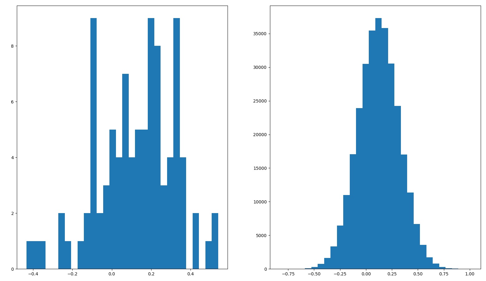 |
| 80% stocks 20% cash | Sampled – 9.7% Normalized – 9.7% | Sampled – 15.6% Normalized – 15.7% | 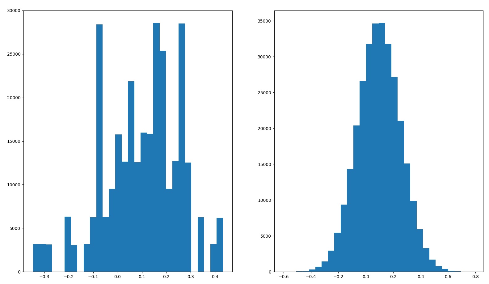 |
| 2 alternate universes | Sampled – 12.2% Normalized – 12.2% | Sampled – 13.8% Normalized – 13.9% | 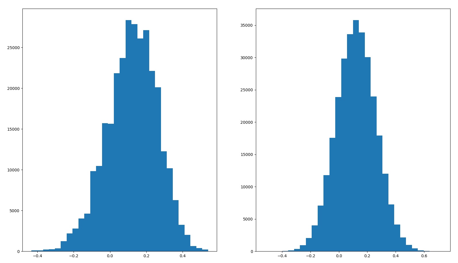 |
| 5 alternate universes | Sampled – 12.1% Normalized – 12.2% | Sampled – 8.75% Normalized – 8.79% | 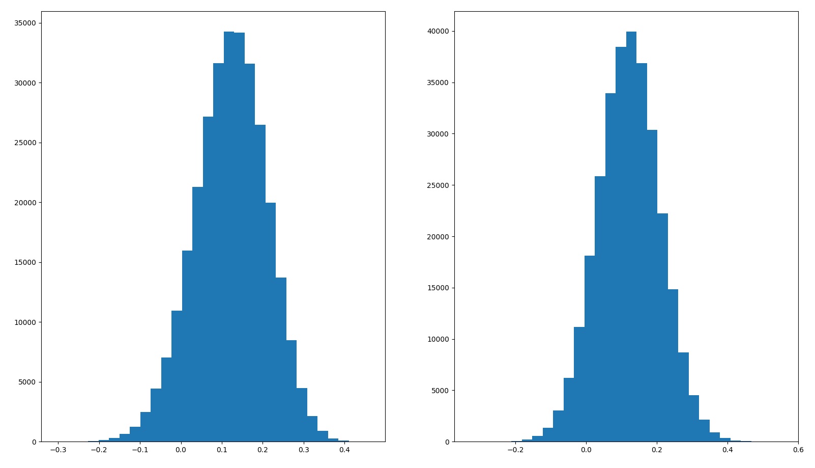 |
| 50% stocks 50% real estate | Sampled – 10.6% Normalized – 10.6% | Sampled – 11.00% Normalized – 11.00% | 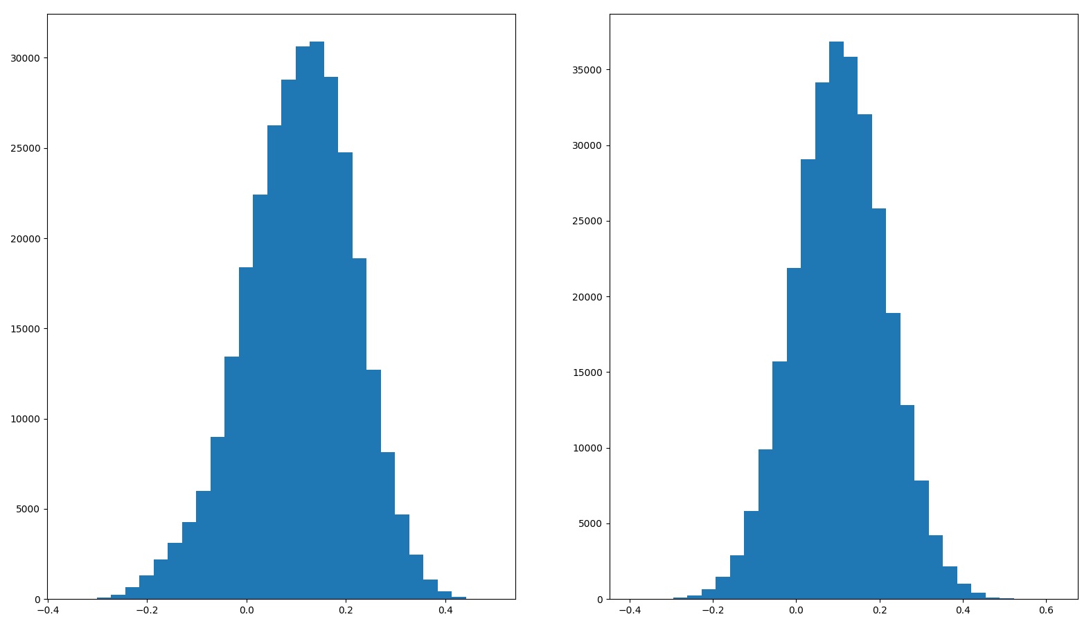 |
And for the same 5 portfolios, we compute the CAGR and SWR over 30 years (see “Monte Carlo” for a full description of the methodology details).
| Portfolio | Average return | Median return | CAGR | SWR 90% | SWR 95% | SWR 99% |
| 100% stocks | Sampled – 12.1% Normalized – 12.1% | Sampled – 13.9% Normalized – 12.1% | Sampled – 10.3% Normalized – 10.4% | Sampled – 3.78% Normalized – 3.95% | Sampled – 3.00% Normalized – 3.25% | Sampled – 1.87% Normalized – 2.08% |
| 80% stocks 20% cash | Sampled – 9.7% Normalized – 9.7% | Sampled – 11.1% Normalized – 9.8% | Sampled – 8.5% Normalized – 8.6% | Sampled – 3.65% Normalized – 3.78% | Sampled – 3.05% Normalized – 3.22% | Sampled – 2.11% Normalized – 2.32% |
| 2 alternate universes | Sampled – 12.2% Normalized – 12.2% | Sampled – 12.9% Normalized – 12.2% | Sampled – 11.3% Normalized – 11.3% | Sampled – 5.42% Normalized – 5.46% | Sampled – 4.76% Normalized – 4.82% | Sampled – 3.60% Normalized – 3.74% |
| 5 alternate universes | Sampled – 12.1% Normalized – 12.2% | Sampled – 12.4% Normalized – 12.1% | Sampled – 11.8% Normalized – 11.8% | Sampled – 6.74% Normalized – 6.78% | Sampled – 6.26% Normalized – 6.34% | Sampled – 5.39% Normalized – 5.46% |
| 50% stocks 50% real estate | Sampled – 10.6% Normalized – 10.6% | Sampled – 11.2% Normalized – 10.6% | Sampled – 10.1% Normalized – 10.0% | Sampled – 5.27% Normalized – 5.29% | Sampled – 4.70% Normalized – 4.81% | Sampled – 3.80% Normalized – 3.93% |
Some interesting results:
- If we invest in 2 or more independent assets, then the sampled returns approximate the normally distributed model.
- This is why the differences between using sampled stock returns and normally distributed model is generally small, especially when we consider a diversified portfolio.
- If you just put 20% of your assets in cash, and 80% in stocks, your expected returns will suffer. However, somewhere in the 95-99%-ile range, your SWR will actually go up.
- If you can invest in stock markets in 2 alternate universes, then your expected annual returns will remain roughly the same. But your CAGR and SWR will increase dramatically.
- This is even more pronounced if you can invest in 5 alternate universes.
- Since I am a mere mortal, the best I can do is invest 50% in stocks and 50% in real estate, which definitely helps SWR, and maybe helps with CAGR as well(3).
Diversification
The basic idea behind the magical increase in CAGR and SWR beyond 100% stocks, is simply “diversification”. When you diversify, and you rebalance your portfolio periodically (4), what you are doing is essentially selling high (the asset which outperformed) and buying low (the asset which underperformed). Buying low and selling high is, historically, the winning strategy for investing (and speculating), and will likely remaining a winning strategy in the future (5).
So, the last problem with the 100% stocks strategy, is that even if real estate has a lower expected annual returns and lower expected CAGR than stocks (3), the very fact that they are not very correlated to stocks means that an allocation to real estate can help increase your portfolio’s CAGR and SWR.
This is the same principle in use when financial advisors recommend investing in index funds (as opposed to single name stocks) — diversification helps to reduce overall volatility and regular rebalancing forces you to buy low and sell high.
Side note: taking profits
A corollary that is not immediately obvious from the above, is the act of “taking profits”. Historically, when people have asked me for advice on what to do after some speculative asset they’ve bought appreciated by a huge amount (more than 100% increase in price), my general advice is something along the lines of “sell enough so that you take a decent profit, and won’t be sad if everything else drops back to your cost basis.”
The psychological effect of doing so is that you’ve now already realized a decent profit, and everything left in that asset is essentially “house money”. While a mathematical fallacy, I have found that this has made holding on to a speculative asset that much easier.
The financial/mathematical effect of doing so, is essentially the same as diversification. Assuming the money you take out is put into another (not very correlated) asset, then you have essentially achieved the “2 alternate universes” scenario.
Code
What kind of a nerd would I be, if I didn’t also present the code for the simulations mentioned above? Note that this builds upon the code in “Monte Carlo” — you’ll need to copy the code there and save it in a file titled “montecarlo.py” for the code below to work.
#!/usr/bin/python3.8

import matplotlib.pyplot as plt
import montecarlo
import numpy


HISTORICAL_RETURNS = montecarlo.HISTORICAL_RETURNS

NormalDistribution = montecarlo.NormalDistribution
UniformSampling = montecarlo.UniformSampling
Cash = montecarlo.Cash
Composite = montecarlo.Composite

GenerateReturns = montecarlo.GenerateReturns
MonteCarlo = montecarlo.MonteCarlo


def PlotHistogram(data):
  _, axs = plt.subplots(1, len(data))
  if len(data) == 1:
    axs.hist(data, bins=30)
  else:
    for i in range(len(data)):
      axs[i].hist(data[i], bins=30)
  plt.show()


def PrintStats(label, data):
  print("{}  Mean:{:.3g}%  StdDev:{:.3g}%".format(
    label,
    numpy.mean(data) * 100,
    numpy.std(data, ddof=1) * 100))


class NormalizedDistribution(NormalDistribution):
  def __init__(self, label, data):
    NormalDistribution.__init__(self, label, numpy.mean(data), numpy.std(data, ddof=1))


def Main():
  cash = Cash("Cash")

  sampled_stocks = UniformSampling("SampledStocks", HISTORICAL_RETURNS)
  normal_stocks = NormalizedDistribution("NormalizedStocks", HISTORICAL_RETURNS)
  normal_re = NormalDistribution("NormalizedRE", 0.09, 0.1)

  data = GenerateReturns(normal_stocks).flatten()
  PrintStats("Historical S&P 500", HISTORICAL_RETURNS)
  PrintStats("Normalized S&P 500", data)
  MonteCarlo(sampled_stocks)
  MonteCarlo(normal_stocks)
  PlotHistogram([HISTORICAL_RETURNS, data])

  sampled_stocks_80 = Composite("80% sampled", (sampled_stocks, 0.8), (cash, 0.2))
  normal_stocks_80 = Composite("80% normalized", (normal_stocks, 0.8), (cash, 0.2))
  s_data = GenerateReturns(sampled_stocks_80).flatten()
  n_data = GenerateReturns(normal_stocks_80).flatten()
  PrintStats("80% sampled stocks, 20% cash", s_data)
  PrintStats("80% normalized stocks, 20% cash", n_data)
  MonteCarlo(sampled_stocks_80)
  MonteCarlo(normal_stocks_80)
  PlotHistogram([s_data, n_data])

  sampled_stocks_alt2 = Composite("Alt2 sampled", (sampled_stocks, 0.5), (sampled_stocks, 0.5))
  normal_stocks_alt2 = Composite("Alt2 normalized", (normal_stocks, 0.5), (normal_stocks, 0.5))
  s_data = GenerateReturns(sampled_stocks_alt2).flatten()
  n_data = GenerateReturns(normal_stocks_alt2).flatten()
  PrintStats("2 alternate universes, sampled stocks", s_data)
  PrintStats("2 alternate universes, normalized stocks", n_data)
  MonteCarlo(sampled_stocks_alt2)
  MonteCarlo(normal_stocks_alt2)
  PlotHistogram([s_data, n_data])

  sampled_stocks_alt5 = Composite("Alt5 sampled",
                                  (sampled_stocks, 0.2), (sampled_stocks, 0.2), (sampled_stocks, 0.2),
                                  (sampled_stocks, 0.2), (sampled_stocks, 0.2))
  normal_stocks_alt5 = Composite("Alt5 normalized",
                                 (normal_stocks, 0.2), (normal_stocks, 0.2), (normal_stocks, 0.2),
                                 (normal_stocks, 0.2), (normal_stocks, 0.2))
  s_data = GenerateReturns(sampled_stocks_alt5).flatten()
  n_data = GenerateReturns(normal_stocks_alt5).flatten()
  PrintStats("5 alternate universes, sampled stocks", s_data)
  PrintStats("5 alternate universes, normalized stocks", n_data)
  MonteCarlo(sampled_stocks_alt5)
  MonteCarlo(normal_stocks_alt5)
  PlotHistogram([s_data, n_data])

  sampled_stocks_re = Composite("Stocks+RE sampled", (sampled_stocks, 0.5), (normal_re, 0.5))
  normal_stocks_re = Composite("Stocks+RE normalized", (normal_stocks, 0.5), (normal_re, 0.5))
  s_data = GenerateReturns(sampled_stocks_re).flatten()
  n_data = GenerateReturns(normal_stocks_re).flatten()
  PrintStats("Sampled stocks + normalized real estate", s_data)
  PrintStats("Normalized stocks + normalized real estate", n_data)
  MonteCarlo(sampled_stocks_re)
  MonteCarlo(normal_stocks_re)
  PlotHistogram([s_data, n_data])


if __name__ == "__main__":
  Main()
Footnotes
- Not religious advice!
- This is an imperfect comparison. The pro forma returns from syndications are estimates and may be wrong (though in my, very limited, experience good sponsors tend to underestimate returns). Also, the pro forma returns of syndications today have very little bearings on historical total returns of real estate over long periods of time. Certainly, the Great Financial Crisis of 2008 taught us that real estate prices can go down too!
- Real estate returns are hard to measure, because real estate tends to illiquid and non-fungible, and the way depreciation affects accounting just confounds that matter even more. The 9% mean, 10% standard deviation modeled here is mostly out of thin air — I picked 9%/10% because it is a lower return with lower volatility than stocks. Some (unverified) data I’ve found suggests this is too pessimistic — historical real estate returns seems to be better than this.
- Rebalancing periodically is key here! If you do not rebalance, then most, if not all, the benefits of diversification goes away. Every time I hear someone boast about how they are both “diversified” and “passive” (so passive that they do not rebalance), I die a little bit inside. I am already old, stop trying to help me along.
- If you’ve managed to lose money by buying low and selling high, please let me know!
