Tag: learning

Foreword

Real estate vs stocks, the perennial debate. Which one should you invest in?

As usual, a reminder that I am not a financial professional by training — I am a software engineer by training, and by trade. The following is based on my personal understanding, which is gained through self-study and working in finance for a few years.

If you find anything that you feel is incorrect, please feel free to leave a comment, and discuss your thoughts.

Caveats

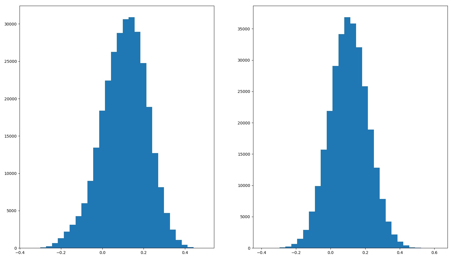
Before we go deeper into the discussion, I’d like to address some criticisms of “Monte Carlo“. To be absolutely clear, in “Monte Carlo” and in this post, I use simplified models to represent returns from various assets. In particular, stock returns have been modeled as normal distributions, which isn’t quite correct:

As you can see from the histograms, actual stock markets total returns (left) is quite different from the stylized normal distribution with similar mean and standard deviation.

Separately, assumptions that stocks and bonds (and in this post, real estate) returns are completely uncorrelated are clearly too permissive. In reality, stocks, bonds and real estate are somewhat (negatively) correlated over short periods of time, as all of them are generally affected by politics, inflation and interest rates, amongst other things.

That said, the point of “Monte Carlo” and this post isn’t to build a perfect model for anyone’s financial planning purposes. Instead, these 2 posts are meant to explore various aspects of portfolio construction — how you should think about expected returns, CAGR, SWR, and how volatility affects these metrics. With this rather more modest goal, I believe the simplified models used are more than adequate.

My my, what low returns you have!

In “My Personal Portfolio“, I mentioned that I invest heavily in real estate, generally via private real estate syndications.

In some private discussions about real estate syndications, others have noted that the pro forma returns presented by some real estate syndications that I invest with (generally in the 10-15% range) are lower than what the stock markets have returned in the past 20 years or so.

If you pick up a calculator, you’ll find that from 2009 – 2020 stocks have returned about 15.5% on average every year, with a CAGR of about 15%. Compared to the 10-15% pro forma returns, it seems silly to even consider real estate.

Therefore, we should just invest 100% in stocks… right?

Expected returns

The first problem with the 100% stocks assertion, is that expected returns are misleading — expected returns are merely “expected” as opposed to “realized”. The future is always uncertain, and it is entirely possible that the next N years see returns dramatically below expected returns based on the past N years.

That is why in “Monte Carlo“, each test is done 10,000 times and the metrics reported are the averages of the 10,000 simulations. However, since the average person cannot live 10,000 lives and pick the best/median/average lives (1), these numbers should be taken with a pinch of salt — they are expected values, not realized nor even predicted values. In the context of a single lifetime, the law of large numbers simply does not hold.

Looking further

The next problem with the 100% stocks assertion is that only looking at the expected returns of the past ~11 years is misleading. Typically, expected returns are the arithmetic means of historical returns. In effect, they tell you “given a random year, what is the expected returns of that year”. Stock markets, however, do not always go up uninterrupted — periods of growth are punctuated with periods of declines.

In the context of historical stock markets performance, the past ~11 years have been unusually kind to stock investors, and it is currently not clear if future years will be as kind.

Since returns are multiplicative, a few years of subpar returns in the future will reduce lifetime CAGR significantly. In “Monte Carlo“, I presented historical total returns of the S&P 500, which suggests that long term CAGR is closer to 10%, with mean annual total returns of around 12.2%. Suddenly real estate is looking much better(2)!

Volatility

As we’ve discussed above and in “Monte Carlo“, volatility in the portfolio, as represented by standard deviation of annual total returns, can dramatically curtail the safe withdrawal rate from that portfolio. To illustrate this point, let’s look at some example scenarios.

In each of these, stocks are represented by both their sampled historical returns as well as their normally distributed returns (mean 12.1%, standard deviation 19.7%). The 2 alternate universes is a hypothetical scenario, where we invest 50% of our portfolio each in 2 completely independent stock markets (i.e.: each stock market in its own alternate universe). 5 alternate universes is where we invest 20% of our portfolio each in 5 completely independent stock markets. Real estate is represented by a normally distributed model with mean of 9% and standard deviation of 10% (3).

In each case, the portfolio is rebalanced annually so that the portfolio is distributed across the assets according to the description.

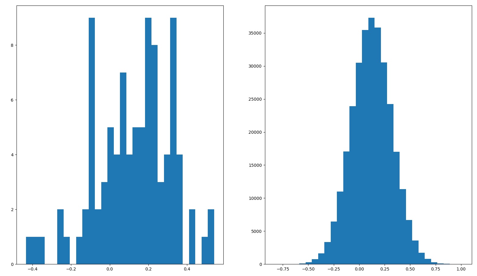
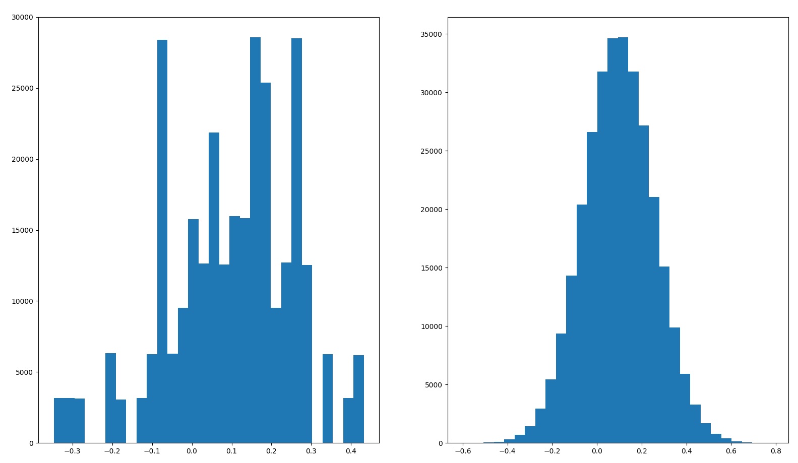
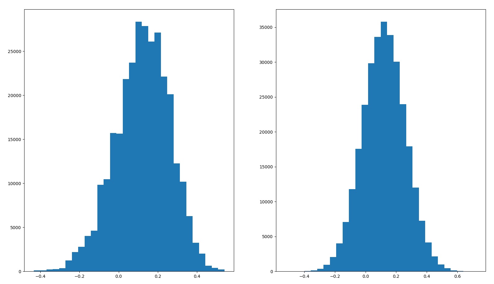
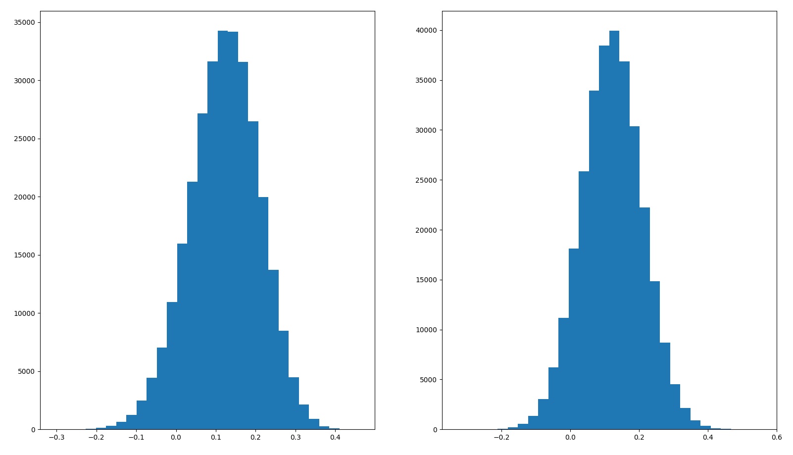
The histogram on the left is when we use sampled historical stock returns for the simulation, and the histogram on the right is when we use normalized stock returns.

Portfolio	Average returns	Standard deviation of returns	Histogram of returns
100% stocks	Sampled – 12.1% Normalized – 12.1%	Sampled – 19.7% Normalized – 19.7%
80% stocks 20% cash	Sampled – 9.7% Normalized – 9.7%	Sampled – 15.6% Normalized – 15.7%
2 alternate universes	Sampled – 12.2% Normalized – 12.2%	Sampled – 13.8% Normalized – 13.9%
5 alternate universes	Sampled – 12.1% Normalized – 12.2%	Sampled – 8.75% Normalized – 8.79%
50% stocks 50% real estate	Sampled – 10.6% Normalized – 10.6%	Sampled – 11.00% Normalized – 11.00%

And for the same 5 portfolios, we compute the CAGR and SWR over 30 years (see “Monte Carlo” for a full description of the methodology details).

Some interesting results:

• If we invest in 2 or more independent assets, then the sampled returns approximate the normally distributed model.
  • This is why the differences between using sampled stock returns and normally distributed model is generally small, especially when we consider a diversified portfolio.
• If you just put 20% of your assets in cash, and 80% in stocks, your expected returns will suffer. However, somewhere in the 95-99%-ile range, your SWR will actually go up.
• If you can invest in stock markets in 2 alternate universes, then your expected annual returns will remain roughly the same. But your CAGR and SWR will increase dramatically.
• This is even more pronounced if you can invest in 5 alternate universes.
• Since I am a mere mortal, the best I can do is invest 50% in stocks and 50% in real estate, which definitely helps SWR, and maybe helps with CAGR as well(3).

Diversification

The basic idea behind the magical increase in CAGR and SWR beyond 100% stocks, is simply “diversification”. When you diversify, and you rebalance your portfolio periodically (4), what you are doing is essentially selling high (the asset which outperformed) and buying low (the asset which underperformed). Buying low and selling high is, historically, the winning strategy for investing (and speculating), and will likely remaining a winning strategy in the future (5).

So, the last problem with the 100% stocks strategy, is that even if real estate has a lower expected annual returns and lower expected CAGR than stocks (3), the very fact that they are not very correlated to stocks means that an allocation to real estate can help increase your portfolio’s CAGR and SWR.

This is the same principle in use when financial advisors recommend investing in index funds (as opposed to single name stocks) — diversification helps to reduce overall volatility and regular rebalancing forces you to buy low and sell high.

Side note: taking profits

A corollary that is not immediately obvious from the above, is the act of “taking profits”. Historically, when people have asked me for advice on what to do after some speculative asset they’ve bought appreciated by a huge amount (more than 100% increase in price), my general advice is something along the lines of “sell enough so that you take a decent profit, and won’t be sad if everything else drops back to your cost basis.”

The psychological effect of doing so is that you’ve now already realized a decent profit, and everything left in that asset is essentially “house money”. While a mathematical fallacy, I have found that this has made holding on to a speculative asset that much easier.

The financial/mathematical effect of doing so, is essentially the same as diversification. Assuming the money you take out is put into another (not very correlated) asset, then you have essentially achieved the “2 alternate universes” scenario.

Code

What kind of a nerd would I be, if I didn’t also present the code for the simulations mentioned above? Note that this builds upon the code in “Monte Carlo” — you’ll need to copy the code there and save it in a file titled “montecarlo.py” for the code below to work.

#!/usr/bin/python3.8

import matplotlib.pyplot as plt
import montecarlo
import numpy


HISTORICAL_RETURNS = montecarlo.HISTORICAL_RETURNS

NormalDistribution = montecarlo.NormalDistribution
UniformSampling = montecarlo.UniformSampling
Cash = montecarlo.Cash
Composite = montecarlo.Composite

GenerateReturns = montecarlo.GenerateReturns
MonteCarlo = montecarlo.MonteCarlo


def PlotHistogram(data):
  _, axs = plt.subplots(1, len(data))
  if len(data) == 1:
    axs.hist(data, bins=30)
  else:
    for i in range(len(data)):
      axs[i].hist(data[i], bins=30)
  plt.show()


def PrintStats(label, data):
  print("{}  Mean:{:.3g}%  StdDev:{:.3g}%".format(
    label,
    numpy.mean(data) * 100,
    numpy.std(data, ddof=1) * 100))


class NormalizedDistribution(NormalDistribution):
  def __init__(self, label, data):
    NormalDistribution.__init__(self, label, numpy.mean(data), numpy.std(data, ddof=1))


def Main():
  cash = Cash("Cash")

  sampled_stocks = UniformSampling("SampledStocks", HISTORICAL_RETURNS)
  normal_stocks = NormalizedDistribution("NormalizedStocks", HISTORICAL_RETURNS)
  normal_re = NormalDistribution("NormalizedRE", 0.09, 0.1)

  data = GenerateReturns(normal_stocks).flatten()
  PrintStats("Historical S&P 500", HISTORICAL_RETURNS)
  PrintStats("Normalized S&P 500", data)
  MonteCarlo(sampled_stocks)
  MonteCarlo(normal_stocks)
  PlotHistogram([HISTORICAL_RETURNS, data])

  sampled_stocks_80 = Composite("80% sampled", (sampled_stocks, 0.8), (cash, 0.2))
  normal_stocks_80 = Composite("80% normalized", (normal_stocks, 0.8), (cash, 0.2))
  s_data = GenerateReturns(sampled_stocks_80).flatten()
  n_data = GenerateReturns(normal_stocks_80).flatten()
  PrintStats("80% sampled stocks, 20% cash", s_data)
  PrintStats("80% normalized stocks, 20% cash", n_data)
  MonteCarlo(sampled_stocks_80)
  MonteCarlo(normal_stocks_80)
  PlotHistogram([s_data, n_data])

  sampled_stocks_alt2 = Composite("Alt2 sampled", (sampled_stocks, 0.5), (sampled_stocks, 0.5))
  normal_stocks_alt2 = Composite("Alt2 normalized", (normal_stocks, 0.5), (normal_stocks, 0.5))
  s_data = GenerateReturns(sampled_stocks_alt2).flatten()
  n_data = GenerateReturns(normal_stocks_alt2).flatten()
  PrintStats("2 alternate universes, sampled stocks", s_data)
  PrintStats("2 alternate universes, normalized stocks", n_data)
  MonteCarlo(sampled_stocks_alt2)
  MonteCarlo(normal_stocks_alt2)
  PlotHistogram([s_data, n_data])

  sampled_stocks_alt5 = Composite("Alt5 sampled",
                                  (sampled_stocks, 0.2), (sampled_stocks, 0.2), (sampled_stocks, 0.2),
                                  (sampled_stocks, 0.2), (sampled_stocks, 0.2))
  normal_stocks_alt5 = Composite("Alt5 normalized",
                                 (normal_stocks, 0.2), (normal_stocks, 0.2), (normal_stocks, 0.2),
                                 (normal_stocks, 0.2), (normal_stocks, 0.2))
  s_data = GenerateReturns(sampled_stocks_alt5).flatten()
  n_data = GenerateReturns(normal_stocks_alt5).flatten()
  PrintStats("5 alternate universes, sampled stocks", s_data)
  PrintStats("5 alternate universes, normalized stocks", n_data)
  MonteCarlo(sampled_stocks_alt5)
  MonteCarlo(normal_stocks_alt5)
  PlotHistogram([s_data, n_data])

  sampled_stocks_re = Composite("Stocks+RE sampled", (sampled_stocks, 0.5), (normal_re, 0.5))
  normal_stocks_re = Composite("Stocks+RE normalized", (normal_stocks, 0.5), (normal_re, 0.5))
  s_data = GenerateReturns(sampled_stocks_re).flatten()
  n_data = GenerateReturns(normal_stocks_re).flatten()
  PrintStats("Sampled stocks + normalized real estate", s_data)
  PrintStats("Normalized stocks + normalized real estate", n_data)
  MonteCarlo(sampled_stocks_re)
  MonteCarlo(normal_stocks_re)
  PlotHistogram([s_data, n_data])


if __name__ == "__main__":
  Main()

Footnotes

1. Not religious advice!
2. This is an imperfect comparison. The pro forma returns from syndications are estimates and may be wrong (though in my, very limited, experience good sponsors tend to underestimate returns). Also, the pro forma returns of syndications today have very little bearings on historical total returns of real estate over long periods of time. Certainly, the Great Financial Crisis of 2008 taught us that real estate prices can go down too!
3. Real estate returns are hard to measure, because real estate tends to illiquid and non-fungible, and the way depreciation affects accounting just confounds that matter even more. The 9% mean, 10% standard deviation modeled here is mostly out of thin air — I picked 9%/10% because it is a lower return with lower volatility than stocks. Some (unverified) data I’ve found suggests this is too pessimistic — historical real estate returns seems to be better than this.
4. Rebalancing periodically is key here! If you do not rebalance, then most, if not all, the benefits of diversification goes away. Every time I hear someone boast about how they are both “diversified” and “passive” (so passive that they do not rebalance), I die a little bit inside. I am already old, stop trying to help me along.
5. If you’ve managed to lose money by buying low and selling high, please let me know!

Foreword

Financial planning, portfolio management and wealth management are often used interchangeably, but they are actually different disciplines in finance.

In this post, we look at the differences between the three, and how they should be employed.

As usual, a reminder that I am not a financial professional by training — I am a software engineer by training, and by trade. The following is based on my personal understanding, which is gained through self-study and working in finance for a few years.

If you find anything that you feel is incorrect, please feel free to leave a comment, and discuss your thoughts.

Financial planning

Financial planning, as the name implies, is a process where you plan out your finances. First, you come up with financial goals that you want to achieve, for example:

• Save for a house down payment by age 30
• Pay for children’s college
• Financial independence by 45
• Retire by 55
• etc.

These goals should have a dollar amount attached, estimated to the best of your abilities. They should also have a deadline. In effect, all of these goals can be translated into a statement of the form:

I want to have $D by year Y.

Once you have your list of goals, you’ll effectively have a list of net worth dollar amounts that you’ll need, by certain years.

The next step is to take stock of what your assets are, right now. You should be able to then assess the viability of your financial plan, by just applying aggressive assumptions for your assets, for example, 15% annual growth year over year, every year. You should also factor in your expected annual income from a job, trust, allowance, etc., as well as your annual expenditures, again, use aggressive assumptions — your income will grow 2-4% a year, your expenditures will only grow 1.5-3% a year, etc.

If your financial plan fails even with the aggressive assumptions, i.e.: you miss one or more goals even with such aggressive assumptions, then your goals are likely unreasonable, and you should re-evaluate the goals and try and make them more reasonable. For example, maybe delaying retirement by a few years?

Finally, you need to figure out how much risk you need to take on, and how much you need to increase your income by, and how much you need to limit your expenditures by, in order to give your financial plan the highest probability of success. This is important! You are not trying to maximize the return of your assets/investments, but rather, under the set of goals, you are trying to figure out what is the least risky way for you to achieve it.

This last step is where you start making more conservative assumptions. Is 15% annual growth in investments reasonable? There certainly are stocks that grow 15% or more a year for long periods of time. But how likely are you to identify them ahead of time? Also, these stocks tend to be more risky — either small/mid caps, highly levered, etc. Also, how likely are you to get a 2-4% raise every year? How much harder will you have to work to achieve that? Are you willing to work that much harder? And how much will you have to sacrifice in terms of living standards to keep your expenditures low? Are you sure you can maintain such low expenditures for long periods of time?

These are all questions you need to ask yourself honestly, and answer honestly. Make the necessary adjustments to what kind of risks you are willing to take with your investments, how much you are willing to put into your job to try and achieve the raises you target, and how much you are willing to forsake in current standards of living in order to meet your goals.

Remember always, that you are trying to maximize the probability that your plan works! Yes, if you work 20hours a day, you may get a 6% raise every year. But is that reasonable? What are the chances that you work yourself into serious health issues, and then have to take months or even years off of work to recover? Think about all these issues, then ask yourself, is it reasonable to expect yourself to work 20hours a day for 2 years? 5 years? 10 years? Probably not!

As you are probably thinking now, this is an iterative process. As you figure out the kind of sacrifices, risks and adjustments you’ll have to make, you’ll find that perhaps you are willing to trade off some goals to reduce the amount of sacrifices, risks and adjustments you’ll need to make, which in turn will likely increase the probability of success.

After a few rounds of adjusting goals, making more conservative assumptions, you’ll have a better picture of the tradeoffs that you need to make — either reducing your goals, or increasing your risk, sacrifices and adjustments.

And once you are done, once you are happy with the final result, you’ll have a financial plan.

That’s not the end, though! Life is unpredictable and things often change without warning. After you have a financial plan, you need to re-evaluate your plan periodically — I like to do it once a year or when I have to make major financial decisions. Figure out if you are on track for your plan, and if not, go through the iterative process again, and figure out what you need to do to get yourself back on track.

Portfolio management

Portfolio management is the curation of your investment assets. For example, let’s say you have a financial plan in place, and you have devoted $100,000 to investing. What assets should you buy? In what ratio? Should you have excess cash lying around to opportunistically time market downturns? Or will you stay 100% invested at all times? Or will you even lever your position to be more than 100% invested?

These are all questions that you’ll answer when you are managing your portfolio.

In order to answer these questions, though, you’ll need to have an idea of the different asset classes. Largely they are:

• Cash
• Equity (stocks, or ownership of private businesses)
• Bonds (or other types of debt(-like) instruments such as loan, preferred equity, etc.)
• Real estate
• Commodities (such as precious metals, agricultural products, energy commodities, or more likely derivatives of these)
• More exotic forms such as fine wine, rare art, etc.

Each of these behave differently in different environments. For example, in inflationary environments, commodities and real estate tends to do well, equity decently, but bonds and cash tend to suffer. In reducing interest rate environments, bonds and equity tend to do well, real estate decently, commodities and cash maybe not so much, etc.

Figuring out what to invest in, and in what ratio, is non-trivial! Happily, for most people, the answer need not be very nuanced. A 60/40 portfolio of 60% equities and 40% bonds (1), with maybe a few percentage taken out of each to invest in real estate will generally be a fairly good trade off between risk undertaken and potential reward. However, if you are willing to spend more time on the topic, you may be able to eek out more return without increasing risk or reduce your risk without reducing your return. Unless you have a substantial amount of assets under you care, however, you may find that the results are simply not worth the effort.

Remember that when you are planning your portfolio, you are effectively aiming for some goal from your financial plan — say you need to get 10% returns every year. This goal may severely hamper the choice of assets that you can invest in! If you aim for 10% returns every year, for example, leaving your portfolio entirely in cash is unlikely to work.

Finally, unlikely financial planning, where the focus is mainly on trying to maximize the probability of success (i.e.: reducing risk), portfolio management takes a more balanced approach and looks more at expected returns of assets, before figuring out how to reconcile that with expected risk (i.e.: trading off risk vs return).

Wealth management

Wealth management is generally spoken of as a service provided by a professional, a wealth manager. It’s not really something someone does for themselves.

In effect, wealth management is a service which combines aspects of financial planning and portfolio management. The wealth manager will work with you to figure out what you are comfortable doing for yourself, and what you would prefer professional help with, and then work through the financial planning and portfolio management process with you. At the extreme, you may simply give the manager power of attorney over your assets, and they will then manage everything towards the goals you’ve discussed, and perhaps send you a regular stipend for living expenses.

In practice, wealth management services tend to be very expensive, as they involve a lot of risk for the manager (legal and liability risks mostly), which need to be defrayed with increased fees. Also, ongoing portfolio management and financial planning services tend to be labor intensive, while also requiring fairly specialized skills, again pointing to high fees. So, in general, wealth management services are typically only offered to those who are wealthy, and for most managers, the minimum assets a client must have is generally in the $2-10m range.

How they intertwine

Financial planning can be thought of as your “life’s goals”, finance-wise. It is the targets that you’d like to hit, if you think of your financial life as a business. Portfolio management is, then, the actual steps you’d take to achieve those targets (though focusing only on investments, while a financial plan often involves incomes and expenditures as well).

Wealth management, in our little analogy, will then be the hiring of external consultants or vendors to advice on or run part of your business for you.

Do I need a financial plan?

Probably yes! Everyone has goals they’d want to meet in the future, and unless you are so incredibly wealthy that almost any goal you can think of can be trivially met financially, you’ll probably want to develop a financial plan to figure out where you stand, and what you need to work on.

Do I need to manage my portfolio?

Probably yes, but this may not be that hard. Unlike financial planning which often involves taking stock of your current situation and trying to figure out what goals are feasible and how much effort/risk you need to take on, portfolio management can be fairly straightforward.

For most people, a passive (or mostly passive) investment portfolio may be appropriate — unless you have specialized knowledge about the financial markets, or you are personally interested in finance, or if you have a large amount of assets already where even a marginal increase in returns is a meaningful absolute number, you may find that effort spent on managing your portfolio to optimize it more, may be wasted. Instead, for most people, it may be more bang-for-the-buck if you spend more of your efforts on trying to increase your income, for example, taking on more at work to aim for a promotion, or taking on a side gig, etc., or by spending time going through your expenses to try and reduce your expenditures.

A passive investment portfolio may be as simple as figuring a ratio between stocks/bonds that you’d like to hold, and then buying the respective indices in the decided ratio. (2)

Do I need a wealth manager?

Probably not. The pre-requisite net worth for a wealth manager to be even willing to work with you is often a bar most people do not meet. And honestly, unless you are incredibly wealthy and have a very complicated financial situation, it probably isn’t worth the money hiring a wealth manager in the first place.

However, if you do happen to have the requisite $2-10m lying around (check your couch!), and you don’t happen to be interested in finance and just want to enjoy what life has to offer, then a wealth manager may indeed be just what you need.

Footnotes

1. For those who are younger, you may want to take on more equity risk, say, 70/30, or even up to 90/10, depending on your risk tolerance. For those who are closer to retirement, you may want to reduce equity risk, say, 50/50, etc.
2. It irks a lot of people, but I generally will not provide financial advice except to people I am close to. This is for conscience reasons (I may be wrong), legal reasons (I am not licensed to provide financial advice) and for liability reasons (you may sue me if I’m wrong). Therefore, this is about as specific as I will go.

Foreword

How much money can you spend every year, if you want your money to last 30 years?

Does this change if you invest 100% in stocks? 100% in bonds? 60/40 in stocks/bonds?

Do you even know what the historical returns of stocks are?

As usual, a reminder that I am not a financial professional by training — I am a software engineer by training, and by trade. The following is based on my personal understanding, which is gained through self-study and working in finance for a few years.

If you find anything that you feel is incorrect, please feel free to leave a comment, and discuss your thoughts.

Raw data

Here is the annual total return (1) of the S&P500 index since 1926, taken from https://www.slickcharts.com/sp500/returns. I haven’t verified the data, but a quick glance suggests it’s probably close enough for our purposes. I’ve excluded 2021 because the year hasn’t ended yet. All numbers are in percentage terms.

  18.40,  # 2020
  31.49,  # 2019
  -4.38,  # 2018
  21.83,  # 2017
  11.96,  # 2016
  1.38,  # 2015
  13.69,  # 2014
  32.39,  # 2013
  16.00,  # 2012
  2.11,  # 2011
  15.06,  # 2010
  26.46,  # 2009
  -37.00,  # 2008
  5.49,  # 2007
  15.79,  # 2006
  4.91,  # 2005
  10.88,  # 2004
  28.68,  # 2003
  -22.10,  # 2002
  -11.89,  # 2001
  -9.10,  # 2000
  21.04,  # 1999
  28.58,  # 1998
  33.36,  # 1997
  22.96,  # 1996
  37.58,  # 1995
  1.32,  # 1994
  10.08,  # 1993
  7.62,  # 1992
  30.47,  # 1991
  -3.10,  # 1990
  31.69,  # 1989
  16.61,  # 1988
  5.25,  # 1987
  18.67,  # 1986
  31.73,  # 1985
  6.27,  # 1984
  22.56,  # 1983
  21.55,  # 1982
  -4.91,  # 1981
  32.42,  # 1980
  18.44,  # 1979
  6.56,  # 1978
  -7.18,  # 1977
  23.84,  # 1976
  37.20,  # 1975
  -26.47,  # 1974
  -14.66,  # 1973
  18.98,  # 1972
  14.31,  # 1971
  4.01,  # 1970
  -8.50,  # 1969
  11.06,  # 1968
  23.98,  # 1967
  -10.06,  # 1966
  12.45,  # 1965
  16.48,  # 1964
  22.80,  # 1963
  -8.73,  # 1962
  26.89,  # 1961
  0.47,  # 1960
  11.96,  # 1959
  43.36,  # 1958
  -10.78,  # 1957
  6.56,  # 1956
  31.56,  # 1955
  52.62,  # 1954
  -0.99,  # 1953
  18.37,  # 1952
  24.02,  # 1951
  31.71,  # 1950
  18.79,  # 1949
  5.50,  # 1948
  5.71,  # 1947
  -8.07,  # 1946
  36.44,  # 1945
  19.75,  # 1944
  25.90,  # 1943
  20.34,  # 1942
  -11.59,  # 1941
  -9.78,  # 1940
  -0.41,  # 1939
  31.12,  # 1938
  -35.03,  # 1937
  33.92,  # 1936
  47.67,  # 1935
  -1.44,  # 1934
  53.99,  # 1933
  -8.19,  # 1932
  -43.34,  # 1931
  -24.90,  # 1930
  -8.42,  # 1929
  43.61,  # 1928
  37.49,  # 1927
  11.62,  # 1926

Pop quiz 1

You can refer to the numbers above, but don’t use a calculator or anything, just try to estimate the answers:

1. What do you think is the average annual return over the period covered?
2. What do you think is the median annual return over the period covered?
3. What do you think is the CAGR(2) over the period covered?
4. Which of the following 3 numbers above should you use, if you want to estimate how much returns you’ll get over the next 10 years?

The answers are:

1. 12.2%
2. 14.3%
3. 10.3%
4. CAGR, because total returns over a period of time compounds multiplicatively. Average and median are non-compounding measures.

Are those numbers surprising? Most people find it surprising that the CAGR is so much lower than the other 2 measures, because they generally hear about the average/median returns thrown around in the media, but CAGR is a number that’s less frequently used, even though it’s more important. Some people, especially those who started investing since 2010, may find it surprising that the numbers are so low, because they are used to 15+% returns, in most years since 2010. However, because returns compound multiplicatively, a down year dramatically skews the CAGR, which is why we see these numbers.

Pop quiz 2

Now, let’s say we have some amount of money, $R, to retire on, and assume inflation rate of 3% (3), which is to say, if you need $X in year one, you’ll need $(1.03 * X) in year 2, and $(1.03^2 * X) in year 3, and so on.

The ratio X/R is your withdrawal rate in the first year. The safe withdrawal rate (or SWR) is the ratio X/R, such that you have a high probability of not running out of money within your retirement — in our case, 30 years.

Assuming we used $R to buy the S&P 500 index on day 1 of our retirement, and ignoring transaction costs, taxes, etc.,

1. What do you think is the SWR if you want a 90% probability of not running out of money in 30 years?
2. What about if we want a 95% probability?
3. 99% probability?

Now, if you are like most people, you’ll probably do something like take average/median/CAGR of stocks return, subtract the inflation rate, and that’s your SWR. That’ll give you a number that is either 9.2%, 11.3% or 7.3%, depending on which measure of stocks return you used.

And all 3 answers are wrong. The correct answers are:

1. 3.8%
2. 3.1%
3. 1.9%

Hopefully, you are surprised (4).

Whadafuqjuzhappened!?

The reason the numbers are so small, is because of volatility. Stocks don’t go up in a straight line, they often take little detours where the annual total returns is the wrong shade of green (5). During the years where stocks are down, you are actually spending a much larger percentage of your assets to maintain your lifestyle — since your spending strictly goes up due to inflation, X/R (or your withdrawal rate) goes up if X goes up and R goes down.

So, if you want to maintain the same lifestyle over time, you’ll need to start off by just withdrawing a smaller portion of your portfolio in the first year, i.e.: a lower SWR, to compensate for these episodic underperformance of stocks.

This is sometimes called “sequencing risk”.

I am never gonna retire

Well, maybe don’t despair yet — it’s not as bad as it sounds. Recall that you don’t have to invest (just) in stocks. You can also invest in bonds! Or real estate! Or fine art! Or in this blog! I take donations! (6)

Now, as we know, bonds have, in recent history, really low yields. At the time of this writing, the 30y US Treasury is yielding only 1.93%. Can bonds really help?

Pop quiz 3

Let’s say you use your entire retirement fund of $R to buy a 30y US Treasury yielding 2% (7). So, what do you think your SWR is for

1. 90% probability of not running out of money in 30 years?
2. 95% probability?
3. 99% probability?

And the answers are… 2.9%. For all 3. Note that we are assuming US Treasuries won’t default, and you’ll always get your money back, on top of all the other assumptions above.

So yea, for 90/95%, it’s not as good as stocks, but the stability of bonds help in the 99% case.

What’s going on here?

Recall that I said the main reason why SWR for stocks is so low, is because of volatility and sequencing risk — you need money every year to survive, even if the stock market is being uncooperative. But bonds, being so helpfully stable (at least in our made up model world with semi-unrealistic assumptions), means that even at 99% (and 100%!) percentile levels, we can have the same SWR of 2.9%, higher, in fact, than their CAGR (which is 2%)!

To hammer home this point, I ran simulations of various scenarios, and the results are summarized below:

“Sampled stocks” is stocks using actual historical returns, uniformly sampled for each simulation year.

“Normalized stocks” is stocks using a random returns sampled from a normal distribution with 12.16% mean and 19.66% standard deviation (which is the mean/standard deviation of our historical data above). As you can see, these numbers are fairly similar. Because it’s easier to model different scenarios using a normal distribution, all other simulations involving stocks use variations of “normalized stocks”.

“Low vol stocks” is stocks where we simply halved the standard deviation for modeling purposes. “Low vol, low return stocks” is stocks where we halved both the standard deviation and the mean. “High vol, high return stocks” is stocks where we doubled both standard deviation and mean.

“2/6/10% bonds” are bonds where the yield is 2%, 6% or 10%. (8)

The remaining rows show composite portfolios where we have some percentage of assets in stocks, bonds or cash, and where we may apply leverage (buying 50% of the portfolio’s value on margin) at different margin interest rates.

Observations

If you go through the data carefully, you’ll quickly see that:

1. Expected returns (either via average, median or CAGR) is not a good predictor of SWR at all, especially at the higher confidences.
2. Instead, volatility, or lack thereof, is a much better predictor of SWR, again, especially at the higher confidences.
3. So, you can sacrifice some expected returns, and get a higher SWR 99% rate, by swapping out some stocks for bonds, or even cash!
4. If you can get cheap leverage, then some mild application of leverage on a balanced portfolio (for example, 60/40 1.5x leverage with 1% margin) can yield even better results.
5. But using leverage without first tamping down volatility is a recipe for disaster (not shown here, but the high vol, high return stocks scenario is a good approximate).

Wrapping up

For a very long time, people have been asking me why I’m “leaving money on the table” by not being more aggressive in stocks, or why I’m not levering 100% into stocks, etc. Some have even suggested a portfolio of 100% UPRO (which is a 3x daily balanced SPY product).

But think of it this way — when you retire, you’ll depend essentially 100% on your portfolio for cashflow to survive. And as we discussed in “net worth“, net worth is only useful if it can be used somehow to generate cash flow. Because, say it with me now, you cannot eat net worth. Therefore, “expected net worth”, based on whatever modeling of expected returns from a risky portfolio, is only useful if I can depend on it, at retirement, to generate cash flow. It doesn’t matter if the expected value of my portfolio is $1B at retirement, if there’s a 50% probability I’d go bankrupt — What? Am I supposed to eat caviar on my mega yacht off Monaco 50% of the time and then jump off a building the other 50%? (9)

What about levering up now and then selling everything at retirement to buy safer assets? Sure, if you happen to retire when the stock markets are at a high. But I’m not inclined to time my retirement based on the whims of the stock market. Also, since I don’t have a crystal ball, that means I’ll have to go with a more conservative strategy.

Which is to say, in general, as you approach retirement, it is a good idea to reduce volatility in your portfolio, so that you can smooth out market madness and thus achieve a higher level of stable cash flow (higher SWR) from your portfolio. (10)

Monte Carlo

By now, you’re probably wondering why this post is titled “Monte Carlo”. That’s simply the name of the methodology I used to run the simulation for the numbers above. The code for the simulation is attached, feel free to play with the assumptions yourself to see what comes up.

Note that for all the stocks based portfolios, the inputs are random (which is why we need Monte Carlo in the first place), so your numbers may differ slightly. But I’ve found that the differences are relatively minor, typically in the 5-10bps range.

#!/usr/bin/python3.8

import numpy


# Number of times to run each simulation.
TOTAL_ITERATIONS = 10000
# Ratio of runs where we must end up with more than $0, before we consider the test a success.
THRESHOLDS = [0.9, 0.95, 0.99, 1]

# Number of years to run for in each simulation.
NUM_YEARS = 30
# Inflation rate of cash withdrawal.
INFLATION = 0.03

# This should be mostly irrelevant.  Just use a large number.
START_CASH = 1000000

# Data from https://www.slickcharts.com/sp500/returns
HISTORICAL_RETURNS = numpy.array([
  18.40,  # 2020
  31.49,  # 2019
  -4.38,  # 2018
  21.83,  # 2017
  11.96,  # 2016
  1.38,  # 2015
  13.69,  # 2014
  32.39,  # 2013
  16.00,  # 2012
  2.11,  # 2011
  15.06,  # 2010
  26.46,  # 2009
  -37.00,  # 2008
  5.49,  # 2007
  15.79,  # 2006
  4.91,  # 2005
  10.88,  # 2004
  28.68,  # 2003
  -22.10,  # 2002
  -11.89,  # 2001
  -9.10,  # 2000
  21.04,  # 1999
  28.58,  # 1998
  33.36,  # 1997
  22.96,  # 1996
  37.58,  # 1995
  1.32,  # 1994
  10.08,  # 1993
  7.62,  # 1992
  30.47,  # 1991
  -3.10,  # 1990
  31.69,  # 1989
  16.61,  # 1988
  5.25,  # 1987
  18.67,  # 1986
  31.73,  # 1985
  6.27,  # 1984
  22.56,  # 1983
  21.55,  # 1982
  -4.91,  # 1981
  32.42,  # 1980
  18.44,  # 1979
  6.56,  # 1978
  -7.18,  # 1977
  23.84,  # 1976
  37.20,  # 1975
  -26.47,  # 1974
  -14.66,  # 1973
  18.98,  # 1972
  14.31,  # 1971
  4.01,  # 1970
  -8.50,  # 1969
  11.06,  # 1968
  23.98,  # 1967
  -10.06,  # 1966
  12.45,  # 1965
  16.48,  # 1964
  22.80,  # 1963
  -8.73,  # 1962
  26.89,  # 1961
  0.47,  # 1960
  11.96,  # 1959
  43.36,  # 1958
  -10.78,  # 1957
  6.56,  # 1956
  31.56,  # 1955
  52.62,  # 1954
  -0.99,  # 1953
  18.37,  # 1952
  24.02,  # 1951
  31.71,  # 1950
  18.79,  # 1949
  5.50,  # 1948
  5.71,  # 1947
  -8.07,  # 1946
  36.44,  # 1945
  19.75,  # 1944
  25.90,  # 1943
  20.34,  # 1942
  -11.59,  # 1941
  -9.78,  # 1940
  -0.41,  # 1939
  31.12,  # 1938
  -35.03,  # 1937
  33.92,  # 1936
  47.67,  # 1935
  -1.44,  # 1934
  53.99,  # 1933
  -8.19,  # 1932
  -43.34,  # 1931
  -24.90,  # 1930
  -8.42,  # 1929
  43.61,  # 1928
  37.49,  # 1927
  11.62,  # 1926
])
HISTORICAL_RETURNS /= 100

# Uncomment to print average, median and CAGR of HISTORICAL_RETURNS.
#print(numpy.mean(HISTORICAL_RETURNS) * 100)
#print(numpy.median(HISTORICAL_RETURNS) * 100)
#print((numpy.prod(HISTORICAL_RETURNS + 1) ** (1 / len(HISTORICAL_RETURNS)) - 1) * 100)


class Sim():
  def __init__(self, label):
    self.__label = label

  def Name(self):
    return self.__label


class FixedRate(Sim):
  def __init__(self, label, interest_rate):
    Sim.__init__(self, label)
    self.__interest_rate = interest_rate

  def Return(self):
    return self.__interest_rate


class NormalDistribution(Sim):
  def __init__(self, label, mean, std_dev):
    Sim.__init__(self, label)
    self.__mean = mean
    self.__std_dev = std_dev

  def Return(self):
    return max(-1, numpy.random.normal(self.__mean, self.__std_dev))


class UniformSampling(Sim):
  def __init__(self, label, data):
    Sim.__init__(self, label)
    self.__data = data

  def Return(self):
    return numpy.random.choice(self.__data)


class Cash(FixedRate):
  def __init__(self, label):
    FixedRate.__init__(self, label, 0)


class FullLoss(FixedRate):
  def __init__(self, label):
    FixedRate.__init__(self, label, -1)


class Composite(Sim):
  def __init__(self, label, *args):
    Sim.__init__(self, label)
    self.__args = args

  def Return(self):
    result = 0
    for asset, ratio in self.__args:
      result += asset.Return() * ratio
    return result


def RunOneIteration(model, rate, returns):
  value = START_CASH
  required_cash = START_CASH * rate
  for i in range(NUM_YEARS):
    if value < required_cash:
      return False
    value -= required_cash
    value *= 1 + returns[i]
    required_cash *= (1 + INFLATION)
  return True


def RunSim(threshold, model, rate, returns):
  num_pass_required = TOTAL_ITERATIONS * threshold
  for i in range(TOTAL_ITERATIONS):
    if RunOneIteration(model, rate, returns[i]):
      num_pass_required -= 1
      if num_pass_required <= 0:
        return True
  return False


def GenerateReturns(model):
  output = numpy.empty([TOTAL_ITERATIONS, NUM_YEARS])

  for i in range(TOTAL_ITERATIONS):
    curr_results = output[i]
    for j in range(NUM_YEARS):
      curr_results[j] = model.Return()

  return output


def Report(model, output):
  print("{}:".format(model.Name()))

  while output:
    prefix = output[:5]
    output = output[5:]
    print("  " + "  ".join(["{:>8s}: {:<7s}".format(metric, "{:.2f}%".format(result * 100)) for (metric, result) in prefix]))
  print()



def MonteCarlo(model):
  returns = GenerateReturns(model)

  highest_rate = {}
  for threshold in THRESHOLDS:
    highest_rate[threshold] = float("nan")
    min_rate = 0
    max_rate = 1
    while round(min_rate, 4) < round(max_rate, 4):
      rate = (min_rate + max_rate) / 2
      if RunSim(threshold, model, rate, returns):
        min_rate = rate
        highest_rate[threshold] = rate
      else:
        max_rate = rate

  output = [
    ("Average", numpy.mean(numpy.mean(returns, axis=1))),
    ("Median", numpy.mean(numpy.median(returns, axis=1))),
    ("CAGR", numpy.mean(numpy.prod(returns + 1, axis=1) ** (1 / NUM_YEARS) - 1)),
  ]

  for threshold, rate in highest_rate.items():
    output.append(("SWR-{}%".format(int(threshold * 100)), rate))

  Report(model, output)


def MakeLabelParams(label, *params):
  full_label = label
  first = True
  for param in params:
    if first:
      first = False
      full_label += " {:.2f}".format(param * 100)
    else:
      full_label += "/{:.2f}".format(param * 100)

  return full_label, *params


def Main():
  cash = Cash("Cash")
  margin = FullLoss("MarginCost")

  bonds2 = FixedRate("2% Bonds", 0.02)
  MonteCarlo(bonds2)

  bonds6 = FixedRate("6% Bonds", 0.06)
  MonteCarlo(bonds6)

  bonds10 = FixedRate("10% Bonds", 0.1)
  MonteCarlo(bonds10)

  sampled_stocks = UniformSampling("SampledStocks", HISTORICAL_RETURNS)
  MonteCarlo(sampled_stocks)

  stocks_mean = numpy.mean(HISTORICAL_RETURNS)
  stocks_stdev = numpy.std(HISTORICAL_RETURNS, ddof=1)
  stocks = NormalDistribution(*MakeLabelParams("Stocks", stocks_mean, stocks_stdev))
  MonteCarlo(stocks)

  low_vol = NormalDistribution(*MakeLabelParams("Stocks[LoVol]", stocks_mean, stocks_stdev * 0.5))
  MonteCarlo(low_vol)

  low_vol_mean = NormalDistribution(*MakeLabelParams("Stocks[LoVolMean]", stocks_mean * 0.5, stocks_stdev * 0.5))
  MonteCarlo(low_vol_mean)

  high_vol_mean = NormalDistribution(*MakeLabelParams("Stocks[HiVolMean]", stocks_mean * 2, stocks_stdev * 2))
  MonteCarlo(high_vol_mean)

  stocks60_bonds240 = Composite("60/40", (stocks, 0.6), (bonds2, 0.4))
  MonteCarlo(stocks60_bonds240)

  stocks55_bonds235_cash10 = Composite("55/35/10", (stocks, 0.55), (bonds2, 0.35), (cash, 0.1))
  MonteCarlo(stocks55_bonds235_cash10)

  # 50% margin loan, at 1% rate = 0.05% interest payments per year.
  stocks60_bonds240_x15 = Composite("60/40 x1.5", (stocks, 0.9), (bonds2, 0.6), (margin, 0.005))
  MonteCarlo(stocks60_bonds240_x15)

  # 50% margin loan, at 6% rate = 3% interest payments per year.
  stocks60_bonds240_x15 = Composite("60/40 x1.5", (stocks, 0.9), (bonds2, 0.6), (margin, 0.03))
  MonteCarlo(stocks60_bonds240_x15)


if __name__ == "__main__":
  Main()

Footnotes

1. Total return is equal to dividends + gains in asset price.
2. CAGR is “compounded annual growth rate”, which is, loosely speaking, the geometric mean of the returns, expressed in percentage terms.
3. I’ve been using 3% for modeling inflation for a while now. People used to laugh at me for this, especially during the 2009-2019 period. After 2020, they are still laughing at me. But for very different reasons. For those who are more conservative, feel free to jack up the value to 5% (or more!) in the simulation to see how that affects the numbers.
4. Look, buddy. I worked really hard to build up the suspense and everything. At least act surprised.
5. Also known as “red”.
6. I’m kidding, I don’t take donations.
7. I’m using 2% because it’s easier to type than 1.93%. Also, US Treasuries have some tax advantages, so it’s probably not THAT crazy an assumption. Finally, there are other “safe’ish” assets that can yield as high as 5-6% “safely”.
8. Yes, 6% and 10% bonds sound crazy in today’s low interest rates world. But there are assets (mostly for accredited investors) which can indeed yield up to 12%. They have varying degrees of risk, and certainly aren’t risk free like this modeling suggests. But they behave very similarly to bonds.
9. Interestingly, someone made the argument to me recently that if there’s an asset with a 25% probability of 10x, and 75% probability of going to 0, the expected value is still 2.5x, which means (paraphrased) “you almost have an obligation to buy that asset”. Hopefully this post and the discussion have shown that the question (and thus answer) is not so simple, and that there are a lot of other considerations other than “expected return”.
10. There are other withdrawal strategies that try to mitigate the sequencing risk issue. Most of them revolve around reducing your cash flow in bad market years (e.g.: keeping your withdrawal rate the same, or even reducing it). Some of them may work, but in general, I’m not really inclined to eat lobster one year and starve the next, just because the stock market decides to tank. I’d rather just have my daily, stable supply of ramen noodle.

Foreword

Contrary to the perception of many people, a lot of things go into a good trading strategy.

It is not simply just “a good idea”, but really, the orchestration of many different disciplines towards a common goal.

As usual, a reminder that I am not a financial professional by training — I am a software engineer by training, and by trade. The following is based on my personal understanding, which is gained through self-study and working in finance for a few years.

If you find anything that you feel is incorrect, please feel free to leave a comment, and discuss your thoughts.

Investing vs Speculating

Before we begin, let’s address the elephant in the room. Are we talking about investing or speculating?

Both. While most associate “trading” with speculation, in this particular post, I’m using the word in a more mechanical way — a “trade” is just a transaction, an exchange, in this case, of cash for some asset.

In the world of speculation, a “successful trade” is actually 2 (or more) separate trades — one or more to get into the “position”, and one or more to get out of it, sometimes also called a “roundtrip”. A speculative trade is never a success until you close out the position.

In the world of investing, most “successful trades” are also “roundtrips”. However, there is a separate class of trade which are perpetual, or near perpetual, where a “successful trade” is simply how you edge into a long term advantageous position. Recall that when investing, you are hoping to profit off the productive capacity of the asset. Therefore, a successful long term trade could simply just be getting into a long position with an asset that is productive and stable, at a good price — in such a trade, you are not looking to sell, instead, you are looking to hold the asset for an indefinite amount of time and let the productive capacity accrue profits.

There is an old trader’s adage which goes roughly, “An investment is a trade gone pear shaped”. And therein lies the difference as explained above, albeit with a tragicomedy twist.

Components of a trading strategy

So what are the components of a trading strategy? In broad terms, a good trading strategy should always have these 3 main components:

• Base thesis
  • Why are we even considering this trade?
  • What is the catalyst, or driver for this trade to perform well?
  • Examples:
    • Inflation trade, e.g.: we believe inflation is going up/down over the next N months/years
    • Macro trade, e.g.: we believe this country/industry/sector will go up/down over the next N months/years because of <reason>
• Execution
  • How would we translate the base thesis, from a purely analytical state, to one or more trades?
  • Embedded in this, are considerations such as:
    • Time horizon – How long are we holding the position in each roundtrip?
    • Instrument – What asset are we going to trade to express the base thesis?
    • Price – At what price are we looking to trade?
    • Trading – Are we going to edge into the position slowly? Or buy everything at once?
  • Example:
    • Base thesis: We believe that inflation will go up slightly in the next 2-3 years
    • Time horizon: 2-3 years
    • Instruments:
      • Short short/medium term Treasuries
      • Long stocks of businesses with fixed input costs and variable output prices
    • Price: At the market based on trading strategy.
    • Trading: Form a basket of the instruments with some ratio, rebalance every 3 months
• Risk management
  • How would we know that our base thesis/execution strategy was wrong?
  • And if one (or both) was wrong, what are we going to do to salvage the situation?
  • Example (follow up on the above):
    • We’ll know our inflation thesis is wrong if inflation does not go up at least 0.1% on a year over year basis every month for the next 6 months.
    • If our thesis is wrong, immediately close out the short Treasuries leg of the position, keep the long stock leg as long as it is still performing at or near broad market performance, and slowly close it out over 2-3 quarters.
    • We’ll know our execution strategy is wrong if inflation does go up as described, but out position does not appreciate faster than broad market performance over a 1 month moving window, sampled daily.
    • If our execution strategy is wrong, immediately close out all positions and rethink.

Case study – Inflation in the 1970s

Base thesis

We are currently in 1971, we predict inflation is going to be much higher for the rest of the decade into 1980.

Execution strategy

Buy near month exchange traded gold futures, and continually roll the contracts forward until expiration of thesis. We believe market pricing is currently fair, so we’ll trade at the market.

We’ll leverage our position by 3x of equity, rebalanced yearly.

Case study result

Anyone who predicted (in 1971) that high inflation will be a problem that decade would have been absolutely correct — inflation went from around 5% in 1971 to 12% in 1975, and finally around 14% in 1980.

However, this simple summary is misleading. Inflation actually fell after 1971 to a low of around 3% in mid 1972, before its enormous rise to 12% in 1975. After that, it again fell to around 5% in 1977, before another huge surge, before ending at around 14% in 1980.

So while the base thesis was, on the whole, correct, the sampling period and how we decide we were correct or wrong (risk management) may have led to us conclude that high inflation was over in 1972 or 1977!

The execution strategy, on the other hand, likely would have given us a roller coaster ride. From 1971 to 1975, gold prices raised from around $260 per ounce to $929 in early 1975. At 3x leverage balanced yearly, we’d have suffered a devastating 91% loss in 1976, ending up with a value worse than if we had simply just bought gold outright without leverage:

If we had closed our position then, however, we’d have lost out on a magnificent rise in value till 1980. True, it’s quite a bit less than 3x what the underlying did, but it was still pretty decent!

The astute reader will notice that in the case study, a section on risk management was left out. This is intentional, because since we are looking at the data in hindsight, any risk management strategy can be crafted to make any arbitrary point. That said, a good risk management strategy would hopefully have gotten us out of the trade either in 1972 (because the base thesis, at that point in time, looked like it might have been wrong), or in mid 1975, because gold prices and inflation were both turning down, or (albeit a very risky strategy) it could have given us the courage to held on to our convictions till 1980.

Why bother?

The reason why a good trading strategy plans out the base thesis, execution strategy and risk management way before even entering a trade, is so that these decisions can be made with a level head. Imagine if you were the portfolio manager of the strategy above. Would you have the conviction to hold in 1972, after a very decent (almost double) gain, but with inflation lower than expected? What about in 1976, after a devastating 91% drawdown? Or would you have folded, expecting gold prices to go even lower (as it did the next year by 1977, by another 12.8%)?

Laying out your strategies, and putting them to paper while you still have a clear head helps to eliminate emotional biases that creep in in the heat of the moment. This gives you a chance to at least think clearly about the issues, and decide what your risk tolerances are.

Foreword

This post discusses some common techniques on evaluating the fundamental value of a company by looking at its cash flow statement, for those who are investing, as defined in Investing vs Speculating.

There are, of course, other ways of evaluating the value of a company, which we will cover in other posts. Other posts in this series:

• How to value a company – income statement
• How to value a company – balance sheet

As usual, a reminder that I am not a financial professional by training — I am a software engineer by training, and by trade. The following is based on my personal understanding, which is gained through self-study and working in finance for a few years.

If you find anything that you feel is incorrect, please feel free to leave a comment, and discuss your thoughts.

Show me the money

If, after reading How to value a company – income statement, you come away thinking there’s way too many finance gobbledygook in there about stuff that aren’t really about cold hard cash, like depreciation, accounts payable, etc., and you’d really just want to figure out whether cash is coming in or leaving the registers. Then you may be tempted to just throw away the income statement and just scream, “Show me the money!”

And you wouldn’t be alone.

This is where the cash flow statement comes in. As the name implies, it is, literally, a statement of the cash flowing into and out of the company. Gone are the hand-wavy “assets” and “costs” like accounts receivable and depreciation. Gone are the confusing terms like “operating costs”, which for some reason, don’t include the costs of actually producing the products (what’s up with that?). Everything is broken down into 5 very simple lines, which tell you exactly how much cash is coming into (or leaving!) the company’s coffers and where they are from (or are going).

Common accounting terms

There’s really only 5 lines on the cash flow statements that are important. Yes, there are probably like 30 lines on an actual cash flow statement (we’ll get to them later), but the 5 important lines are:

Showing your work

Yes, there’s really only 5 lines that matter. But you know how things are. We can’t make life too simple — where’s the fun in that? In general, a cash flow statement will contain, oh, about 30-50 lines. The lines other than the 5 lines mentioned above, are basically just the accountants showing their work.

Like in elementary school math, where you can’t just write “5”, or even “The answer is 5”. No, you have to write:
Sally has 2 marbles. Peter has 3 marbles. Total marbles = 2 + 3 = 5.

The result is the same. But the teachers prefer the latter. It makes them feel happier. Or something.

This is good for us! Sometimes the accountants (or the company itself) get things wrong. So they show their work on the cash flow statement. And we get to decide if they know how to do basic arithmetic. (1)

One thing to note: numbers in parentheses are negative numbers — cash flowing out of our company. For example, in the “cash from financing activities” section, “(5,000)” generally means we paid off $5,000 in debt. The parentheses means cash flowing out, and numbers without parentheses mean cash coming in.

And now what?

From the cash flow statement, we can discern a few very important tidbits:
Is most of the cash coming into the company via actual operations?
Or is the company being propped up by more and increasing debt?
Or by selling off assets?

Ideally, we want “total cash from operations” to be a positive number, and much larger than “total cash from investing” and “total cash from financing”.

Even better if “total cash from financing” is a negative number (we are doing so well, we can pay down debt!). Note that a positive “total cash from financing” number isn’t necessarily a bad thing. Maybe the company is raising debt to buy out a competitor and thus expanding its businesses. Or maybe the company is developing a new product line, etc. One off debt issuance to invest into the business is usually a good thing! The red flag is when “total cash from financing” is always positive (i.e: the company is always issuing debt), and always a substantial amount compared to “total cash from operations”.

“Total cash from investing” should hopefully also be a negative number, indicating the business is likely profitable and the company is investing more money into it. However, this is more nuanced.

If “total cash from investing” is always negative, and always a large absolute number, that may indicate a business that is heavily dependent on new injections of capital. For example, if a company has $1,000,000 of “total cash from operations” every quarter, but also $(900,000) of “total cash from investing” every quarter, that suggests that perhaps the company is heavily dependent on rolling over its investments every period to generate the profits for the next period.

Companies like this are sometimes at the mercy of their customers — if they also have a large accounts receivable, if their customers fail to pay up on time, these companies may get into temporary liquidity distress.

Even without being at the mercy of their customers, these companies generally don’t tend to perform as well — the need for heavy capital reinvestment makes it hard to scale the business, because it is not always possible to find enough capital to deploy; At the same time, the need for heavy capital investment (as a ratio of operating profits) suggests lower profitability, which deters investors.

Free cash flow

Free cash flow tells us the core efficiency of a company’s businesses — It is simply the cash the operations of a company generate, without consideration for reinvestments (i.e.: capital expenditure).

Recall that “total cash from operations” is the cash a company generates ignoring depreciation and amortization (amongst other things). So, by starting with “total cash from operations”, we just need to take out “capital expenditure” to get free cash flow:

“Capital expenditure” is the amount of cash a company reinvests in its businesses. For example, to replace capital assets that were consumed as part of operations, or to scale the business. This is sometimes called out in the cash flow statement or income statement, but usually needs to be estimated or calculated — by looking at the income statement and deducing which line items are related to capital expenditure.

Free cash flow = total cash from operations - capital expenditure

Another form of free cash flow, unlevered free cash flow, is simply free cash flow assuming the company has no debt. In this case, interest expenses are added back to the value of “free cash flow”, while tax breaks for interest expenses are taken out:

Unlevered free cash flow = free cash flow + interest expenses - tax deductions due to interest expenses

Note that tax deductions due to interest expenses may not appear in the cash flow statement nor the income statement, and may have to be estimated.

Free cash flow essentially tells us “how much this company can return if we just run it ‘into the ground'”, i.e.: without replacing consumed capital assets. It is a base case of what profits the company is capable of extracting from its businesses.

Unlevered free cash flow is similar, and gives us an idea of what free cash flow would look like, if an acquirer buys out the company and pays off all its debts.

There are other variants of free cash flow that are sector specific. The most widely used is “funds from operations”, which is used commonly in real estate heavy companies (such as REITs). “Funds from operations” is just unlevered free cash flow with losses and gains from sale of properties removed, i.e.: gains are taken out, losses are added back in. The idea is similar — to try and get a number that gives us an idea how profitable this company can be, purely from its core operations.

Once we have determined the variant of free cash flow we are using, and have computed its value, the next question is, what do we do with this number?

Recall that free cash flow gives us an idea of the core efficiency of a company at its businesses. So the most common thing, is to look at free cash flow over time. Is it consistently going up? Is it growing at a suitable rate based on investments into the businesses? How much is the shareholder paying for each dollar of free cash flow?

Ideally, we want free cash flow to be increasing over time, and at a pace equal or faster than reinvestment rate — if the company is reinvesting profits equal to 20% of capital assets, then free cash flow should increase by 20% or more in subsequent periods (2). Otherwise, the company would probably be better off investing that money in other pursuits, or returning the cash to investors.

Sometimes, an unprofitable company may be a good investment, even if free cash flow is currently negative! A company that is heavily investing in its businesses may sometimes have negative free cash flow — recall that free cash flow is operating cash flow – capital expenditure. Assuming the capital expenditure is a temporary event (3), when the need to invest in scaling the business stops, free cash flow will likely quickly jump to positive. Note that such businesses are not without their risks! There is a chance that the capital expenditure does not result in future profits, for example, if the research failed to find anything useful, etc.

Finally, the price / free cash flow (P/FCF) ratio is a useful indicator of how much the investor is paying for dollar of free cash flow from the company. As with the other price ratios (P/E, P/S, etc.), the numerator is usually the market capitalization (price per share can also be used if free cash flow is also normalized to free cash flow per share).

Like the P/S ratio, the P/FCF ratio may be useful for informing whether a company is a good investment at a certain price, even if the company is currently unprofitable. Furthermore, the P/FCF ratio is also useful for companies that have strong and stable cash flows (such as some real estate related businesses) — unlike the P/E ratio, the P/FCF (or P/FFO — price per funds from operations) tends to provide a more stable value less affected by one time events that are not related to the core operations.

A company with a good P/FCF ratio, but a terrible P/E ratio may simply be affected by accounting quirks like depreciation and amortization rules, which are not strictly part of the core operations.

Footnotes

1. I kid! Nowadays, every financial statement pushed out by a public company, especially a large, public company, is scrutinized by an army of analysts whose jobs are, in part, to make sure silly arithmetic mistakes are rooted out. The additional lines are still useful for those who are curious, and want to know the breakdown even more, though.
2. Note that in some industries, there is a significant lag time between when investments are made, to when profits from those investments can be extracted. This should be taken into account when judging if free cash flow is growing at a rate commensurate with the investment rate.
3. Many types of businesses are characterized by heavy capital expenditure in a few years, followed by many years of extracting profits from those capital expenditures. For example, research and development heavy industries (pharmaceuticals, some technology firms, etc.), manufacturing industries (building factories, etc.). Once the capital expenditure is done, the company may be able to enjoy many years of profits without having to do more capital expenditure.

Foreword

This post discusses some common techniques on evaluating the fundamental value of a company by looking at its balance sheet, for those who are investing, as defined in Investing vs Speculating.

There are, of course, other ways of evaluating the value of a company, which we will cover in other posts. Other posts in this series:

• How to value a company – income statement
• How to value a company – cash flow statement

As usual, a reminder that I am not a financial professional by training — I am a software engineer by training, and by trade. The following is based on my personal understanding, which is gained through self-study and working in finance for a few years.

If you find anything that you feel is incorrect, please feel free to leave a comment, and discuss your thoughts.

What does a company own?

In the previous post of this series, we considered how a company operates, by looking at its income statement. In this post, we focus instead on what a company is, or more accurately, what it owns.

We have already discussed in the previous post how a model company operates, and how its earnings and sales numbers affect our decision on how much the company is worth. But sometimes, a company does not actually have operations. For example, a holding company is essentially just a legal container that “holds” other companies. The holding company itself has minimal operations — it is mostly only a corporate shell to provide some amount of bookkeeping, legal and financial services to the companies it owns, and it is those companies that have actual businesses and operations.

Trying to value a holding company using P/E ratio, P/S ratio or any metric that falls out of its income statement will necessarily lead to misleading numbers — the main value add of the entire conglomerate is not so much its corporate operations, but the operations of its individual constituent companies.

While we can passthrough the underlying metrics of all the children companies, aggregate them and then compute our valuation ratios based on that, the result is also likely confounding — the children companies may be in different sectors/industries, and at different stages of their corporate lives. Combining revenue and expense numbers across drastically different companies rarely makes a whole lot of sense.

While a holding company is an extreme example, there are certain sectors/industries where purely looking at the income statement of a company can lead to misleading answers. For example, there are companies where a lot of the company’s value is in its assets (such as intellectual property, rights to certain natural resources, actual physical assets that appreciate, etc.), and the assets generally does not depreciate in value quickly (or may even appreciate!). For these companies, even if they do not have any operations, you can make the case that they have value — their assets can be sold or leased to others to generate potential profits.

For companies in these situations, a better way of valuing the company may be to just look at what the company owns — by looking at its balance sheet — and then computing the value of each component and adding them all up.

Common accounting terms

Even in our simple model of a company above, a lot of interesting terms pop up. Understanding how to read a company’s balance sheet will require some basic understanding of these terms.

Note that balance sheets tend to be more freeform, with companies having a decent amount of leeway of defining line items. Because of this, we’ll only discuss line items that are more common across different companies. Sector/industry/company specific line items tend to be self descriptive.

Useful quick gauges

Reading the numbers

The numbers and ratios that we can compute based on the balance sheet generally does not translate directly into a value we should pay for a company. Remember that what a company owns, is not reflective of its potential (or lack thereof!). It is the operations that management layers on top of the company’s assets that generates profits — simply gathering a bunch of factory equipment and putting them together does exactly nothing.

Therefore, except for the special case of a company where operations are to be wound up (e.g: when management is so inept that the best use of the company’s resources is to sell them off and return the cash to shareholders), the balance sheet mostly just tells us how well run a company is, how efficient it is, how profitable is its business, and all of these in terms of the inputs (i.e: funding via equity and debt) into the company.

A well run company will generally have a respectable ROE and ROIC. Generally somewhere in the 10% range is considered pretty good. This is not a hard and fast rule! There are some businesses that are naturally welcoming of leverage, and these tend to have very low ROIC (though potentially very high ROE). For example, most forms of real estate and banking businesses tend to have rather low ROIC because they are so leveraged. In fact, some publishers of company statistics don’t even publish ROIC for banks, because the number is so misleading.

Therefore ROE and ROIC tend to be sector/industry specific — certain sectors/industries just tend to have companies with higher or lower ROE/ROIC.

At the same time, Quick, Current as well as debt to capital ratios give us an idea of how indebted a company is, how likely it is able to service its debts with cash flow, and how likely it is able to meet short term obligations. These are generally useful only on a company by company basis — they tell us how healthy the company is, and how worried we should be of losing our investments in that company.

Finally, the P/B ratio tells us how much we are paying for the company’s assets. It is meaningful only between companies in the same sector/industry, as well as maturity (recall that younger companies tend to have different operating characteristics from more mature ones).

By themselves, none of these metrics are particularly useful for valuing a company. However, they can be used to supplement what we know from the company’s income statement. For example, a company with a particularly high ROE/ROIC for its sector/industry may command a higher P/E (or P/S or whatever) ratio.

Footnotes

1. Notice how this goes back to the investing vs speculating argument — productive assets, used to generate future investment returns vs non-productive assets, used to generate speculative returns.
2. This mathematically true, but not practically true. In practice, whenever a company has more debt on its books, the interest rate lenders will demand will go up sharply. At the same time, every business has a natural limit to how much it can grow. If a business is selling to all the customers it can possibly sell to, then increasing operations will not increase profits. For most companies, it is generally true that as investment in the business goes up, the ROIC will fall — another way of saying this is that the marginal profit from the marginal dollar of investment is a diminishing quantity.