Capital Stack

Foreword

How do business ventures get funded? Who’s paying for the overhead when the company is first starting out and has no revenue? And what do they get out of this?

As usual, a reminder that I am not a financial professional by training — I am a software engineer by training, and by trade. The following is based on my personal understanding, which is gained through self-study and working in finance for a few years.

If you find anything that you feel is incorrect, please feel free to leave a comment, and discuss your thoughts.

Decent proposal

Let’s say you have a fantastic new business idea, but to get the business started will require $50,000 right now, which you do not have. How could you fund your new venture?

Traditionally, there are 2 main avenues:

  1. Take a loan from a bank
  2. Take on some partners who have deeper pockets (i.e.: sell a portion of your new company)

The former is also known as debt financing, and the latter is equity financing.

When you take on debt, you agree to pay the lender some amounts of money on some fixed timeline. For example, 1% of the loan amount every month (interest payment), and then 100% of the loan amount at the end of 10 years (principal payment).

When you take on partners, they share in the profits (or losses!) of the entire enterprise. So, if after paying off all your bills (which may include debt payments), you are left with $1,000 to distribute between the partners, then you and your partner can(1) get up to $1,000 in total. Who gets how much depends on your partnership agreement, as well as how much of the company each of you own.

First come, maybe not first served

Who gets how much money, and when, is one of the 2 central differences between debt vs equity financing.

Debts must always be paid back, on the timeline agreed upon when the loan is taken out. If you fail to make even a single payment on the debt, it is technically in default, and may officially be in default after some grace period. At that point, the lender generally has some set of rights they can exercise, up to and including forcing you to give up ownership of your company to them.

Equity partners, on the other hand, generally have no fixed payments due. A company can very well never return a single cent to the equity partners! The main considerations are the partnership agreement(2), which will detail how any payments, if made, will be distributed amongst the partners, and fairness — in general, in the absence of any details about how profits are shared, then all dividends will be made pro rata, i.e.: if each of the partners own 50% of the company, then every dollar distributed will see 50c go to each partner.

One way of thinking about this, is that debt investors have the first dibs on revenue generated by the business. Once all debt payments are made, and all other costs are paid, whatever is left over (which may be nothing, or even negative — a loss) can be distributed to the equity partners. In exchange for this “seniority” in terms of payment, debt investors typically settle for a smaller and shorter-term profit — interest rates are generally much lower than what the business can be expected to return over the long term.

Control your enthusiasm

The other central difference between debt and equity financing is that of control, or rather rights — who has rights to do what with the company?

Debt investors generally have no rights on the company other than their regular payments (sometimes known as coupons). If, however, a payment was missed for long enough that the company is in default of the loan agreement, then debt investors generally have additional rights to recover their investment, such as forcing the equity partners to give up ownership of the company, or forcing a sale of the business to 3rd parties to repay the loan.

Equity investors are generally split into 2 groups — the general partners(3) who oversee the actual running of the company, and may even be personally responsible if the company goes bankrupt, and the limited partners, who generally provide the funding for the business, but otherwise have no say in the day to day running of the company.

Mix ‘n match

When you think carefully about it, debt investors and equity investors are very similar at a very high level. Each of them:

  • Provide capital for a company …
  • … and, in return, receives some promise of cash flow at a future time, …
  • … along with some rights with regards to the company.

And at this abstract level, it shouldn’t be surprising, then, to learn that the tradition little boxes that debt and equity investors fit in, are not nearly that clean cut in practice.

In practice, an investor in a company is labeled debt or equity based mostly on their rights to call an event of default on the company. If an investor can call an event of default on the company when their promised distribution is not received, then they are typically labeled debt investors. Otherwise, they are an equity investor.

Some examples, in order of decreasing priority when profits are being distributed (i.e.: an investor at a lower row is not paid, until all investors in higher rows are paid according to the agreement):

Senior debtTypically the highest priority of debt investor. All coupons of senior debt must generally be paid, before anyone else sees a single cent.

Due to this priority, senior debt is typically much safer than all other tiers of investors, and in many cases, senior debt investors may even have collateral — assets owned by the company which the investor can seize if the loan is in default.

In exchange for these protections, senior debt tends to have the lowest interest rates (i.e.: the lowest returns).
Mezzanine debtNot often seen, except in very large projects with huge capital requirements.

Mezzanine debt are paid after senior debt, but before all else. In most cases, mezzanine debt either are exactly the same as senior or junior debt, except that they are paid in between the two.

The additional carveout is almost always entirely just to provide the payment priority protection, and thus a higher interest rate than senior debt, but a lowest interest rate than junior debt.
Junior debtWhen there are 2 (or more) classes of debt investors, the lowest tier is called junior debt.

Junior debt typically are more risky, as they are paid only after senior/mezzanine debts are paid. Also, junior debt typically don’t have collateral.

In exchange for the increased risk, junior debt tends to command the highest interest rates of all debt tiers.
Preferred equityPreferred equity can really be anything at all — anything that you can describe in a legal contract (the partnership agreement) is probably fair game.

In some cases, preferred equity share the same uncertain returns as equity, but are paid first in cases of bankruptcies (i.e.: their entire investment is returned to them, and whatever is left is distributed to the equity tier).

Most commonly, however, preferred equity are very similar to debt — they get a fixed coupon that is generally at a higher rate than junior debt, and they may get a little bit extra if the business does exceptionally well.

In exchange for this higher rate of interest, preferred equity gives up the right to call an event of default on the company if their coupons are not made on time.
EquityThe equity tier is typically the lowest priority in terms of distribution of profits. This means that if there isn’t enough money to satisfy the claims of all higher priority tiers, the equity tier may not get any profits at all. However, if the business does exceptionally well, then the equity tier may get a return much higher than all other tiers combined.

The equity tier is also commonly known as “share holders” (or “stock holders”). When you buy and sell a stock, say GOOG, on the public markets, you are essentially trading ownership interests of the equity tier of that company.

A table where a company lists all its debt and equity investors, according to their priority in terms of payment and their contributions to the venture, is called a “capitalization table” (or “cap table” for short). A table or description detailing how the profits are actually distributed (assuming there are any profits to distribute) is called the “waterfall”.

In general, as you go down a cap table, risk increases, but potential return also increases.

To each their own

Which tier you want to invest in, is entirely up to you and your personal situation.

If you are a retiree, and you need stability of income, you may opt to give up some upside, but get more protection by going up the capital stack (i.e.: going up the rows in the cap table).

But if you are investing for the long term, and you are diversified such that your investment in a single company is a relatively small part of your entire portfolio, then it may make sense to take on the additional risks involved in the lower tiers, for a chance at a higher return — even if this particular company goes bankrupt and you lose all your money in it, hopefully, enough other companies that you’ve also invested in will succeed, such that you still make a greater return than investing at a higher tier.

In the end, where each investor ends up on the capital stack depends on their expectations of how the company will perform, as well as their personal financial situation (generally, their ability to withstand uncertain cash flow and/or losses).

Footnotes

  1. “Can”, not “will”, because in most cases, distributions (or dividends) are not paid on new companies. New companies tend to be very cash hungry, as they need cash to spin up their factories, advertising, research, etc., and more cash is almost always better. As such, equity partners generally don’t tend to see a single cent of profits until years 2-3 or beyond. The exact timeline depends on the nature of the business — some cash intensive businesses may not see a dividend for decades!
  2. Technically, a “partnership agreement” is only used in a partnership (this is a legal term). LLC’s (limited liability company) and corporations use “operating agreements” instead. However, for purely financing purposes, the basic principles remain the same — a group of people got together to fund the equity tier of a company, and there’s a document that describes what they can expect to get out of that venture. I’ll use partnerships for simplicity going forward. Understand that the issues discussed affects LLC’s and corporations as well, though perhaps with minor differences.
  3. As with “partnership agreement”, “general partner” and “limited partner” are terms used in partnerships (the legal entity). LLC’s and corporations have different names for these roles (board of directors, executive team vs shareholders, etc.). Despite the naming differences, the roles are mostly the same and for simplicity, I’ll stick with the nomenclature for partnerships.
Diversification

Foreword

Real estate vs stocks, the perennial debate. Which one should you invest in?

As usual, a reminder that I am not a financial professional by training — I am a software engineer by training, and by trade. The following is based on my personal understanding, which is gained through self-study and working in finance for a few years.

If you find anything that you feel is incorrect, please feel free to leave a comment, and discuss your thoughts.

Caveats

Before we go deeper into the discussion, I’d like to address some criticisms of “Monte Carlo“. To be absolutely clear, in “Monte Carlo” and in this post, I use simplified models to represent returns from various assets. In particular, stock returns have been modeled as normal distributions, which isn’t quite correct:

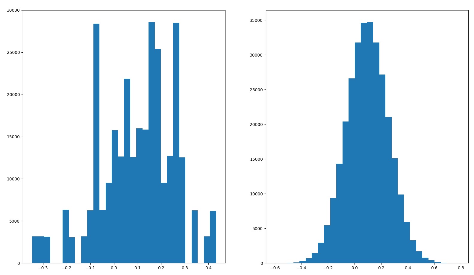
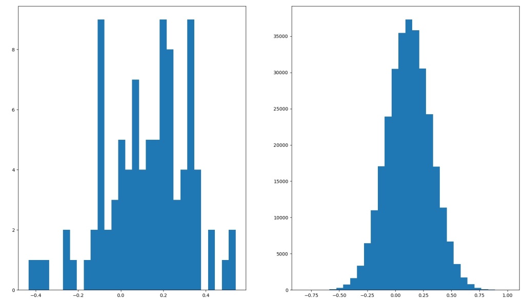
Left: Historical total returns of S&P500 from 1926 to 2020, inclusive.
Right: Normal distribution with 12.2% mean returns and 19.7% standard deviation.

As you can see from the histograms, actual stock markets total returns (left) is quite different from the stylized normal distribution with similar mean and standard deviation.

Separately, assumptions that stocks and bonds (and in this post, real estate) returns are completely uncorrelated are clearly too permissive. In reality, stocks, bonds and real estate are somewhat (negatively) correlated over short periods of time, as all of them are generally affected by politics, inflation and interest rates, amongst other things.

That said, the point of “Monte Carlo” and this post isn’t to build a perfect model for anyone’s financial planning purposes. Instead, these 2 posts are meant to explore various aspects of portfolio construction — how you should think about expected returns, CAGR, SWR, and how volatility affects these metrics. With this rather more modest goal, I believe the simplified models used are more than adequate.

My my, what low returns you have!

In “My Personal Portfolio“, I mentioned that I invest heavily in real estate, generally via private real estate syndications.

In some private discussions about real estate syndications, others have noted that the pro forma returns presented by some real estate syndications that I invest with (generally in the 10-15% range) are lower than what the stock markets have returned in the past 20 years or so.

If you pick up a calculator, you’ll find that from 2009 – 2020 stocks have returned about 15.5% on average every year, with a CAGR of about 15%. Compared to the 10-15% pro forma returns, it seems silly to even consider real estate.

Therefore, we should just invest 100% in stocks… right?

Expected returns

The first problem with the 100% stocks assertion, is that expected returns are misleading — expected returns are merely “expected” as opposed to “realized”. The future is always uncertain, and it is entirely possible that the next N years see returns dramatically below expected returns based on the past N years.

That is why in “Monte Carlo“, each test is done 10,000 times and the metrics reported are the averages of the 10,000 simulations. However, since the average person cannot live 10,000 lives and pick the best/median/average lives (1), these numbers should be taken with a pinch of salt — they are expected values, not realized nor even predicted values. In the context of a single lifetime, the law of large numbers simply does not hold.

Looking further

The next problem with the 100% stocks assertion is that only looking at the expected returns of the past ~11 years is misleading. Typically, expected returns are the arithmetic means of historical returns. In effect, they tell you “given a random year, what is the expected returns of that year”. Stock markets, however, do not always go up uninterrupted — periods of growth are punctuated with periods of declines.

In the context of historical stock markets performance, the past ~11 years have been unusually kind to stock investors, and it is currently not clear if future years will be as kind.

Since returns are multiplicative, a few years of subpar returns in the future will reduce lifetime CAGR significantly. In “Monte Carlo“, I presented historical total returns of the S&P 500, which suggests that long term CAGR is closer to 10%, with mean annual total returns of around 12.2%. Suddenly real estate is looking much better(2)!

Volatility

As we’ve discussed above and in “Monte Carlo“, volatility in the portfolio, as represented by standard deviation of annual total returns, can dramatically curtail the safe withdrawal rate from that portfolio. To illustrate this point, let’s look at some example scenarios.

In each of these, stocks are represented by both their sampled historical returns as well as their normally distributed returns (mean 12.1%, standard deviation 19.7%). The 2 alternate universes is a hypothetical scenario, where we invest 50% of our portfolio each in 2 completely independent stock markets (i.e.: each stock market in its own alternate universe). 5 alternate universes is where we invest 20% of our portfolio each in 5 completely independent stock markets. Real estate is represented by a normally distributed model with mean of 9% and standard deviation of 10% (3).

In each case, the portfolio is rebalanced annually so that the portfolio is distributed across the assets according to the description.

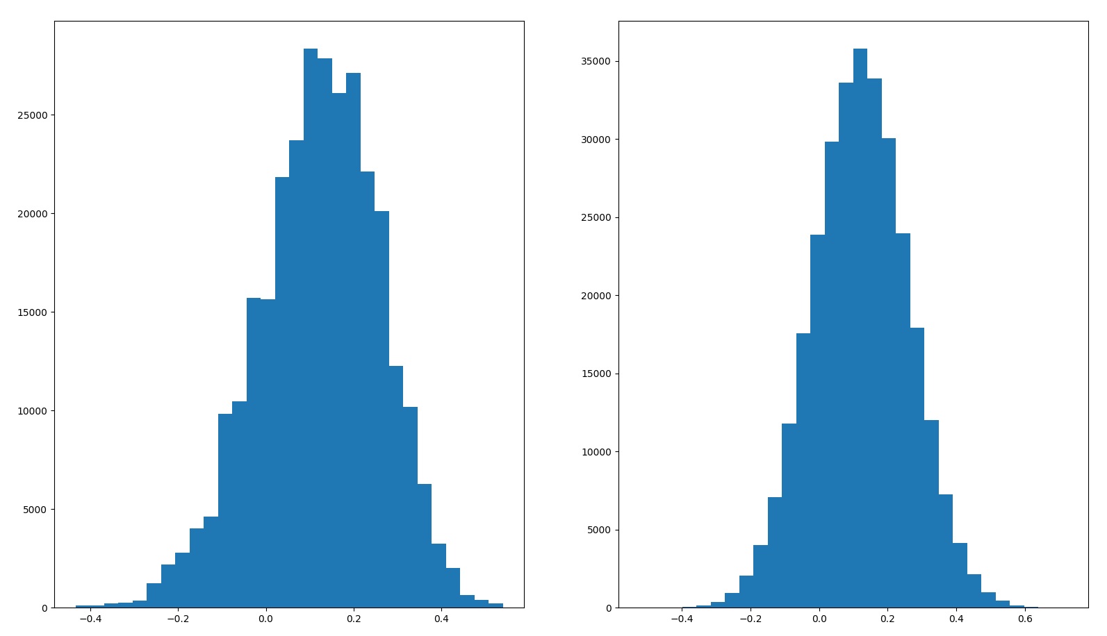
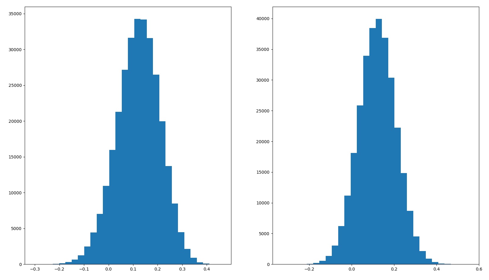
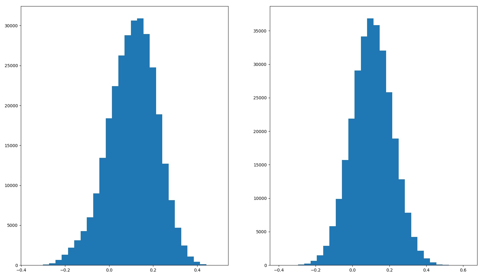
The histogram on the left is when we use sampled historical stock returns for the simulation, and the histogram on the right is when we use normalized stock returns.

PortfolioAverage returnsStandard deviation of returnsHistogram of returns
100% stocksSampled – 12.1%
Normalized – 12.1%
Sampled – 19.7%
Normalized – 19.7%
80% stocks 20% cashSampled – 9.7%
Normalized – 9.7%
Sampled – 15.6%
Normalized – 15.7%
2 alternate universesSampled – 12.2%
Normalized – 12.2%
Sampled – 13.8%
Normalized – 13.9%
5 alternate universesSampled – 12.1%
Normalized – 12.2%
Sampled – 8.75%
Normalized – 8.79%
50% stocks 50% real estateSampled – 10.6%
Normalized – 10.6%
Sampled – 11.00%
Normalized – 11.00%

And for the same 5 portfolios, we compute the CAGR and SWR over 30 years (see “Monte Carlo” for a full description of the methodology details).

PortfolioAverage returnMedian returnCAGRSWR 90%SWR 95%SWR 99%
100% stocksSampled – 12.1%
Normalized – 12.1%
Sampled – 13.9%
Normalized – 12.1%
Sampled – 10.3%
Normalized – 10.4%
Sampled – 3.78%
Normalized – 3.95%
Sampled – 3.00%
Normalized – 3.25%
Sampled – 1.87%
Normalized – 2.08%
80% stocks 20% cashSampled – 9.7%
Normalized – 9.7%
Sampled – 11.1%
Normalized – 9.8%
Sampled – 8.5%
Normalized – 8.6%
Sampled – 3.65%
Normalized – 3.78%
Sampled – 3.05%
Normalized – 3.22%
Sampled – 2.11%
Normalized – 2.32%
2 alternate universesSampled – 12.2%
Normalized – 12.2%
Sampled – 12.9%
Normalized – 12.2%
Sampled – 11.3%
Normalized – 11.3%
Sampled – 5.42%
Normalized – 5.46%
Sampled – 4.76%
Normalized – 4.82%
Sampled – 3.60%
Normalized – 3.74%
5 alternate universesSampled – 12.1%
Normalized – 12.2%
Sampled – 12.4%
Normalized – 12.1%
Sampled – 11.8%
Normalized – 11.8%
Sampled – 6.74%
Normalized – 6.78%
Sampled – 6.26%
Normalized – 6.34%
Sampled – 5.39%
Normalized – 5.46%
50% stocks 50% real estateSampled – 10.6%
Normalized – 10.6%
Sampled – 11.2%
Normalized – 10.6%
Sampled – 10.1%
Normalized – 10.0%
Sampled – 5.27%
Normalized – 5.29%
Sampled – 4.70%
Normalized – 4.81%
Sampled – 3.80%
Normalized – 3.93%

Some interesting results:

  • If we invest in 2 or more independent assets, then the sampled returns approximate the normally distributed model.
    • This is why the differences between using sampled stock returns and normally distributed model is generally small, especially when we consider a diversified portfolio.
  • If you just put 20% of your assets in cash, and 80% in stocks, your expected returns will suffer. However, somewhere in the 95-99%-ile range, your SWR will actually go up.
  • If you can invest in stock markets in 2 alternate universes, then your expected annual returns will remain roughly the same. But your CAGR and SWR will increase dramatically.
  • This is even more pronounced if you can invest in 5 alternate universes.
  • Since I am a mere mortal, the best I can do is invest 50% in stocks and 50% in real estate, which definitely helps SWR, and maybe helps with CAGR as well(3).

Diversification

The basic idea behind the magical increase in CAGR and SWR beyond 100% stocks, is simply “diversification”. When you diversify, and you rebalance your portfolio periodically (4), what you are doing is essentially selling high (the asset which outperformed) and buying low (the asset which underperformed). Buying low and selling high is, historically, the winning strategy for investing (and speculating), and will likely remaining a winning strategy in the future (5).

So, the last problem with the 100% stocks strategy, is that even if real estate has a lower expected annual returns and lower expected CAGR than stocks (3), the very fact that they are not very correlated to stocks means that an allocation to real estate can help increase your portfolio’s CAGR and SWR.

This is the same principle in use when financial advisors recommend investing in index funds (as opposed to single name stocks) — diversification helps to reduce overall volatility and regular rebalancing forces you to buy low and sell high.

Side note: taking profits

A corollary that is not immediately obvious from the above, is the act of “taking profits”. Historically, when people have asked me for advice on what to do after some speculative asset they’ve bought appreciated by a huge amount (more than 100% increase in price), my general advice is something along the lines of “sell enough so that you take a decent profit, and won’t be sad if everything else drops back to your cost basis.”

The psychological effect of doing so is that you’ve now already realized a decent profit, and everything left in that asset is essentially “house money”. While a mathematical fallacy, I have found that this has made holding on to a speculative asset that much easier.

The financial/mathematical effect of doing so, is essentially the same as diversification. Assuming the money you take out is put into another (not very correlated) asset, then you have essentially achieved the “2 alternate universes” scenario.

Code

What kind of a nerd would I be, if I didn’t also present the code for the simulations mentioned above? Note that this builds upon the code in “Monte Carlo” — you’ll need to copy the code there and save it in a file titled “montecarlo.py” for the code below to work.

#!/usr/bin/python3.8

import matplotlib.pyplot as plt
import montecarlo
import numpy


HISTORICAL_RETURNS = montecarlo.HISTORICAL_RETURNS

NormalDistribution = montecarlo.NormalDistribution
UniformSampling = montecarlo.UniformSampling
Cash = montecarlo.Cash
Composite = montecarlo.Composite

GenerateReturns = montecarlo.GenerateReturns
MonteCarlo = montecarlo.MonteCarlo


def PlotHistogram(data):
  _, axs = plt.subplots(1, len(data))
  if len(data) == 1:
    axs.hist(data, bins=30)
  else:
    for i in range(len(data)):
      axs[i].hist(data[i], bins=30)
  plt.show()


def PrintStats(label, data):
  print("{}  Mean:{:.3g}%  StdDev:{:.3g}%".format(
    label,
    numpy.mean(data) * 100,
    numpy.std(data, ddof=1) * 100))


class NormalizedDistribution(NormalDistribution):
  def __init__(self, label, data):
    NormalDistribution.__init__(self, label, numpy.mean(data), numpy.std(data, ddof=1))


def Main():
  cash = Cash("Cash")

  sampled_stocks = UniformSampling("SampledStocks", HISTORICAL_RETURNS)
  normal_stocks = NormalizedDistribution("NormalizedStocks", HISTORICAL_RETURNS)
  normal_re = NormalDistribution("NormalizedRE", 0.09, 0.1)

  data = GenerateReturns(normal_stocks).flatten()
  PrintStats("Historical S&P 500", HISTORICAL_RETURNS)
  PrintStats("Normalized S&P 500", data)
  MonteCarlo(sampled_stocks)
  MonteCarlo(normal_stocks)
  PlotHistogram([HISTORICAL_RETURNS, data])

  sampled_stocks_80 = Composite("80% sampled", (sampled_stocks, 0.8), (cash, 0.2))
  normal_stocks_80 = Composite("80% normalized", (normal_stocks, 0.8), (cash, 0.2))
  s_data = GenerateReturns(sampled_stocks_80).flatten()
  n_data = GenerateReturns(normal_stocks_80).flatten()
  PrintStats("80% sampled stocks, 20% cash", s_data)
  PrintStats("80% normalized stocks, 20% cash", n_data)
  MonteCarlo(sampled_stocks_80)
  MonteCarlo(normal_stocks_80)
  PlotHistogram([s_data, n_data])

  sampled_stocks_alt2 = Composite("Alt2 sampled", (sampled_stocks, 0.5), (sampled_stocks, 0.5))
  normal_stocks_alt2 = Composite("Alt2 normalized", (normal_stocks, 0.5), (normal_stocks, 0.5))
  s_data = GenerateReturns(sampled_stocks_alt2).flatten()
  n_data = GenerateReturns(normal_stocks_alt2).flatten()
  PrintStats("2 alternate universes, sampled stocks", s_data)
  PrintStats("2 alternate universes, normalized stocks", n_data)
  MonteCarlo(sampled_stocks_alt2)
  MonteCarlo(normal_stocks_alt2)
  PlotHistogram([s_data, n_data])

  sampled_stocks_alt5 = Composite("Alt5 sampled",
                                  (sampled_stocks, 0.2), (sampled_stocks, 0.2), (sampled_stocks, 0.2),
                                  (sampled_stocks, 0.2), (sampled_stocks, 0.2))
  normal_stocks_alt5 = Composite("Alt5 normalized",
                                 (normal_stocks, 0.2), (normal_stocks, 0.2), (normal_stocks, 0.2),
                                 (normal_stocks, 0.2), (normal_stocks, 0.2))
  s_data = GenerateReturns(sampled_stocks_alt5).flatten()
  n_data = GenerateReturns(normal_stocks_alt5).flatten()
  PrintStats("5 alternate universes, sampled stocks", s_data)
  PrintStats("5 alternate universes, normalized stocks", n_data)
  MonteCarlo(sampled_stocks_alt5)
  MonteCarlo(normal_stocks_alt5)
  PlotHistogram([s_data, n_data])

  sampled_stocks_re = Composite("Stocks+RE sampled", (sampled_stocks, 0.5), (normal_re, 0.5))
  normal_stocks_re = Composite("Stocks+RE normalized", (normal_stocks, 0.5), (normal_re, 0.5))
  s_data = GenerateReturns(sampled_stocks_re).flatten()
  n_data = GenerateReturns(normal_stocks_re).flatten()
  PrintStats("Sampled stocks + normalized real estate", s_data)
  PrintStats("Normalized stocks + normalized real estate", n_data)
  MonteCarlo(sampled_stocks_re)
  MonteCarlo(normal_stocks_re)
  PlotHistogram([s_data, n_data])


if __name__ == "__main__":
  Main()

Footnotes

  1. Not religious advice!
  2. This is an imperfect comparison. The pro forma returns from syndications are estimates and may be wrong (though in my, very limited, experience good sponsors tend to underestimate returns). Also, the pro forma returns of syndications today have very little bearings on historical total returns of real estate over long periods of time. Certainly, the Great Financial Crisis of 2008 taught us that real estate prices can go down too!
  3. Real estate returns are hard to measure, because real estate tends to illiquid and non-fungible, and the way depreciation affects accounting just confounds that matter even more. The 9% mean, 10% standard deviation modeled here is mostly out of thin air — I picked 9%/10% because it is a lower return with lower volatility than stocks. Some (unverified) data I’ve found suggests this is too pessimistic — historical real estate returns seems to be better than this.
  4. Rebalancing periodically is key here! If you do not rebalance, then most, if not all, the benefits of diversification goes away. Every time I hear someone boast about how they are both “diversified” and “passive” (so passive that they do not rebalance), I die a little bit inside. I am already old, stop trying to help me along.
  5. If you’ve managed to lose money by buying low and selling high, please let me know!

My Personal Portfolio

Foreword

This is a discussion of how I think about my personal portfolio, and what I do with it.

I want to be absolutely clear here — this post is about me, myself and I, and nobody else. What I do for my portfolio may or may not be suitable for anyone else, especially you. I am not a trained financial analyst, financial planner nor financial anything — please consult a professional if you need help with your own financial planning and/or portfolio management.

If you find anything that you feel is incorrect, please feel free to leave a comment, and discuss your thoughts.

Conservative overall portfolio

Firstly, let’s get this out of the way — I am a scaredy cat. I am not trying to become a billionaire — my financial plan resolves entirely around early retirement, paying for my children’s college degrees and leaving them enough assets to bootstrap their adult lives. So, my investment choices generally tend towards more conservative assets, which as we’ve discussed before, are expected to provide more stable cash flows and allow for a higher safe withdrawal rate.

Ballast portfolio

I’m not sure where I first heard the term “ballast”, but it refers to the part of the portfolio that forms the “foundation” or “fallback” — if everything else goes to smelly, this is the part that will likely remain, relatively unscathed. A long time ago (does anyone still remember pre-QE days?), this part of my portfolio was just US Treasury bonds and municipal bonds. They provide a very safe, but lower, yield, which I can generally depend upon.

However, with the advent of QE, these bonds yield too little to be meaningful, yet are priced so richly that even a relatively small increase in interest rates(1) will cause their current mark-to-market values to plummet. As such, they went from “safe, but lower yield” to “risky, and essentially no yield”. Not really what I would call ballast-material!

In place of government bonds, I have been trying various other assets to form the ballast of my portfolio. For now(2), I have settled on these:

  1. Private real estate equity funds
  2. Various short term bonds (of both government and corporate varieties)
  3. Short term private notes

The main goal of the ballast portfolio is to provide a source of stable cash flow, from which to fund all other endeavors.

Stocks portfolio

Other than the ballast side of my portfolio, everything else is invested in stocks. In my stocks portfolio, I further divide into 3 accounts:

  1. Ballast-lite
  2. Main
  3. Gamble

Ballast-lite account

The ballast-lite account of my stocks portfolio is, as its name implies, allocated in safer, more conservative stocks and strategies. For example,

  1. Stable, conservative dividend stocks
  2. Index funds with the wheel strategy(3)

Like the ballast portfolio, the goal is for stable growth, with relatively controlled downside.

Main account

The main account of my stocks portfolio is where I do what most people do (or should do) in the bulk of their portfolios — buy index funds and mostly forget about it. In this account, I also buy some blue chip stocks that I’ve done research on, and are willing to hold for the long term.

Generally, I buy the stocks outright, though for the single name stocks, I may use the wheel strategy to tamp down on volatility and/or squeeze out some additional yield.

Gamble account

The gamble account of my stocks portfolio is where I do crazy things. This is a relatively small account, where I try out experimental strategies, or just bet on silly things (I’ve bought and sold puts and calls on GME during the Jan-Mar 2021 madness).

This is also the account I generally use when I’m uncomfortable about the market, and just want to hedge some of the exposure in the other accounts — in that case, I’ll buy some puts or even outright short in this account to counterbalance the stock exposures in the other accounts.

Target proportions

Ultimately, the goal is for the ballast portfolio to yield enough cash flow to support my lifestyle (with inflation adjusted), while remaining under 50% of my investable assets. When that happens, I’ll know that I can comfortably and safely retire.

The ballast-lite account is meant to provide additional spending money as a buffer, as well as for splurges — maybe I fancy a new flashy car, or to go on an exotic vacation, etc. The main and the gamble accounts are meant to provide for growth in the overall portfolio, as well as assets to leave to my children.

In my stocks portfolio, I generally keep around 30-45% in the ballast-lite account, 30-45% in the main account, and everything else in the gamble account. The exact ratio depends on their recent performances and how I feel about the market — sometimes I forget to rebalance for months on end.

Final word

As noted before, this is a rather conservative portfolio — most people in their prime working years should probably have less than ~60-70% of their portfolio in “ballast”-like investments(4).

However, I’ve found that this suits me fine — I have a day job that pays reasonably well, and so, for my investments, I prefer surety to higher expected, but much more volatile, returns. If nothing else, it helps me sleep at night.

This, again, may or may not be suitable for you. Please consult a professional advisor if you need help with financial planning.

Footnotes

  1. Recall that the Federal Reserve can, almost unilaterally, increase short term interest rates at will.
  2. As the market environment changes, I may tweak or even completely revamp the assets I hold as ballast. And I almost certainly will not be giving anyone a heads up before I do. Therefore, recall the disclaimer — please consult a professional advisor if you need help with financial planning.
  3. The wheel strategy is where you start by having cash, and writing cash secured puts on the asset. If you don’t get assigned, then you just roll the puts over to the next period. If you get assigned, then you switch to writing stock secured calls. Essentially, this caps your upside, but provides a buffer on the downside before you suffer losses.
  4. In my defense, I’ve found that I’ve consistently managed to squeeze out fairly reasonable returns from the “ballast”-like assets, generally to the tune of around 10%, which as we’ve discussed before, is what stocks generally yield over long periods of time anyway.

Inflation model

Foreword

QE, money printing, fiscal stimulus… inflation?! What is inflation? What determines how high inflation gets?

This is a discussion of my personal model of inflation and how it occurs.

I want to be absolutely clear here — this is based entirely on personal study and understanding — I am not a trained economist. All I have, is a high school diploma(1) in Economics, from over 2 decades ago — no doubt there are gaps and/or flaws in my understanding.

If you find anything that you feel is incorrect, please feel free to leave a comment, and discuss your thoughts.

What is inflation?

First off, let’s define inflation. The official economics definition of inflation has undergone some changes throughout history. In this post, I’ll be using the more common, modern day textbook definition which is roughly: Inflation is the general increase in prices of goods and services, and thus a general decrease in the purchasing value of money.

In the quantity theory of money, the equation of exchange gives us(2):

MV = PT

(Simplified) Equation of exchange, https://en.wikipedia.org/wiki/Equation_of_exchange

where

  • M – The total nominal money supply
  • V – The velocity of money
  • P – Price level
  • T – The number of financial transactions

So, assuming the number of financial transactions is the same, then an increase in P (inflation) is simply an increase in MV.

i.e.: Inflation is a product of increasing total money supply times the velocity of money.

Of particular note, and this is something that a lot of people get wrong — inflation is the increase in general price levels:

  • Inflation is not the increase in price(s) of one or even a handful of products.
    • It needs to be an increase in prices of all or almost all products.
  • Inflation is not high prices.
    • Inflation is the increase in prices.
    • Even if prices are still low after the increase, it is still inflation.
    • Conversely, if prices are high, but didn’t increase, then it is not inflation.
  • If after a round of high inflation (large increases in prices), prices remain stable at very high levels, then inflation did not persist.
    • Just because the effects of inflation are permanent, need not mean that inflation itself is permanent.
    • For prices to go back to “normal” levels, would require negative inflation (decrease in prices), also known as deflation.

Hyperinflation

In today’s financial environment, whenever inflation is brought up, people immediately jump to hyperinflation, conjuring up images in their minds of stacks of useless cash pushed around in wheelbarrows.

To be clear, the official definition of hyperinflation is 50% month over month increases in prices, which translates to around 129x (12974.63%) annually. Compared to that, the current 5-6% annual inflation rate is pretty tame.

That said, what causes hyperinflation? Well, happily(3), history provides a lot of examples of where hyperinflation struck. In the popular retellings of these events, the story generally goes along the lines of, “the government/central bank printed more and more bank notes, resulting in an excessive supply of these notes, which then resulted in their devaluation and thus inflation”.

In my opinion, that is a very misleading description of what transpired. As a thought experiment, imagine if the governments of the hyperinflationary events were to print the bank notes, and then burn them up in a giant bonfire. Do you think there would have been hyperinflation, or even high inflation then? It seems to me, that the excessive printing of money was a necessary, but not sufficient step towards hyperinflation. It was the left out bit, the part where “the government then spent the newly printed money with abandon”, which resulted in hyperinflation. In effect — simply printing the bank notes did nothing. But distributing them via government spending (i.e.: fiscal policy), resulted in the increase of money supply(4) (increase in M), and the excessive spending by the government resulted in more money being spent and circulated (increases in V). And that excessive spending is the actual trigger of hyperinflation.

In simple terms, it is not “printing money” that is the problem, but the attempt at creating “value” out of thin air — by printing bank notes not backed or offset by anything, and then spending them as if they were valuable.

Monetary vs fiscal policy

Just a quick note here, because we are going to talk about monetary and fiscal policies a lot.

Monetary policies are generally policies with regards to the money supply .

Fiscal policies are generally policies with regards to taxation and government spending.

In modern society/finance, you can think of monetary polices loosely as “what central banks decide to do”, and you can think of fiscal policies loosely as “what governments decide to tax and spend on”.

Quantitative easing

Since 2009 when quantitative easing (QE) started in the USA (and most of the world), there have been many analysts going on about how QE is printing money, and that it would result in hyperinflation. These doomsayers make very compelling arguments by equating QE to money printing, conjuring up images of massive industrial printers working overtime. However, it has been over 12 years, and only fairly recently did inflation even get comfortably past the 2% that central banks generally target. What happened?

Facts

Before we discuss what happened with QE, let’s talk about some facts:

  • In the USA, QE started in 2009, and was increase multiple times since then, with the latest increase in around March 2020 due to the Covid-19 pandemic.
  • In the USA, inflation from 2009 to March 2020 has generally been low to very low, generally in the 0-2% range.
  • Most other developed nations saw similar trajectories with regards to QE and inflation as the USA, though numbers and dates may be slightly different.
  • Japan started aggressive monetary policies in the early 90’s, culminating in QE around 2001 — 8 years before most of the other developed nations.
  • Japan’s annual inflation rate up to March 2020 has generally been extremely low, with bouts of deflation (negative inflation).
  • In March 2020, in addition to aggressive monetary policies by central banks around the world, fiscal policies around the world also stepped up, culminating in a series of transfer payments(5) around late 2020 into early 2021.
  • In March 2021, we finally saw inflation pick up in the USA.
  • Again, most of the world mirrored the USA’s experience since 2020.

Printing money

The first thing to note when discussing QE, is that it isn’t really “printing money”. In the popular nomenclature, “printing money” generally implies a(n) (attempted) creation of additional “value” out of thin air. However, that is simply not what QE does.

Imagine if you are a bank and I am a client. I choose to deposit $1000 cash with you. In exchange for my cash, you give me a little deposit slip saying I now have $1000 with you. Now, I can write a check against my $1000 with you, and most places would accept my check as payment for services. In effect, that check is “money”(6), and I have, almost literally, “printed money” (with a pen!). I’m sure we can all agree, that lil’ ol’ me isn’t going to cause inflation, much less hyperinflation.

In technical terms, when I deposit $1000 with you, you created 2 entries in your ledger — one under “assets”, which is the actual $1000 cash I deposited with you. The other entry is under “liabilities”, which is the $1000 you now owe me. The total amount of “value” in the system is the same — the $1000 under your assets cancels out the -$1000 under your liabilities.

In a similar fashion, central banks are the banks of normal banks — normal banks can deposit their money with central banks. Generally, (normal) banks need to put up a certain amount of money with their central banks known as reserves. There are complicated rules around the minimum level of reserves a bank needs, and we won’t go into that here, but basically, for a bank to operate, it needs a certain amount of money in the central bank. Any money the bank has in excess of that reserve requirement, is called “excess reserves”(7).

During the Great Financial Crisis of 2008, a lot of assets held on banks’ balance sheets were deemed “risky”. To avoid bank failures, regulators demand that banks increase their amount of reserves. However, there was a general liquidity crunch at the time, so banks couldn’t really do that. At the time, central banks stepped in, and essentially bought up a lot of these assets on the banks’ balance sheets (generally government debt, and government guaranteed mortgage debts). In some sense, this is the same as me depositing my $1000 with you — the banks give the Federal Reserve assets worth $X(8), and the Federal Reserve give the banks a little deposit slip saying “I now owe you $X” (9). On the Federal Reserve’s books, under “assets”, we have these newly bought assets, and under “liabilities”, we have $X owed to the banks.

As you can see, there isn’t really any attempt to create “value” out of thin air. Yes, in a very literal sense, “money is printed” (via increase in reserves on the banks’ books). But that “money” is really just a matched asset/liability pair on the Federal Reserve’s books, and the net “value” in the system is the same — just as me depositing $1000 with you, and then spending that $1000 via a check doesn’t really create “value”.

Liquidity

After the Great Financial Crisis, central banks continued QE, essentially buying up assets from banks, and increasing banks’ excess reserves account (after the immediate crisis, banks already meet your reserve requirements, so any excess sales of assets to central banks really only increase excess reserves).

A further charge of the doomsayers, is that these excess reserves is money, and thus this “money printing” causes inflation.

As we’ve discussed above, while this is “money printing” in the literal sense, there is no attempt at creating “value” out of thin air unlike hyperinflationary episodes from history, because while the central banks issue (excess) reserves, they also take away “value” by taking away equivalent value in assets.

However, there are some effects of this QE! By buying up assets in a price insensitive manner, the central banks effectively put a floor on the value of some assets (generally safe assets like government bonds and government backed debts). This has 2 effects:

  1. These assets that the central banks target effectively have a higher clearing price (i.e.: become more expensive than they would be without QE).
  2. The money that was previously invested in these assets now need to be invested elsewhere.

Together, this resulted in what is colloquially known as “yield tourism” — investors forced out of safe Treasuries and government backed debts, now have to “reach for yield” by buying more risky assets, such as corporate debt, municipal bonds, equities, etc.

In effect, this increased the liquidity in the system, by both reducing the amount of assets that money can buy, and increasing the amount of money in the system. However, this effect is generally confined to financial markets — the Federal Reserve really isn’t in the market to buy baby diapers or new cars. The money displaced by the Federal Reserve’s buying will generally go into buying other financial assets instead of being spent on consumer goods.

In simple terms, if you’ve $1000 to invest, just because the Federal Reserve prevents you from buying some financial assets, doesn’t mean that you’ll just spend that $1000 on chocolate bars! You will likely just invest in something else — that $1000 doesn’t really make it into the consumer goods market.

Putting it all together

In summary, I believe that QE does not result in inflation. Instead, it results in “financial assets inflation”, which is colloquially used to mean increase in financial asset prices only. This is also why, I believe, the prices of stocks, bonds and various other liquid financial assets have been going up non-stop since 2009.

How then, do we explain the high inflation that started around March 2021? Well, recall under “Facts” above, that QE wasn’t the only thing that happened in 2020. Something else happened. Something new. Something changed in mid/late 2020 — governments started massive fiscal policy programs.

Recall from our short note in “Hyperinflation”(10) how inflation doesn’t really begin until that newly created money is spent. Well, that newly created money started being distributed for spending around mid/late 2020 into early 2021. And then we saw inflation take off in early 2021.

In technical terms, before 2020, while M (the money supply) was rapidly increasing, V (the velocity of money) was rapidly decreasing. As a result, the product MV was actually increasing at a rather slow rate, thus low inflation. After late 2020, the rate at which V decreased slowed down dramatically (it is now almost flat), but M increased dramatically. As a result, MV started increasing at a higher rate, i.e.: higher inflation.

Crimping inflation

Recall that in my August inflation update I noted that I believe the Federal Reserve has all the tools it needs to combat inflation. How would that work if I’m now saying fiscal policy is the cause of inflation?

Well, one way of analogizing about this is that loose monetary policy is fuel, and loose fiscal policy is heat. You cannot start a fire with only fuel, and you cannot start a fire with only heat. You need to combine both(11) to start a fire.

Which is to say, I believe that the Federal Reserve can clamp down on inflation by simply tightening monetary policies — inflation can be reduced by simply reducing money supply faster than the velocity of money. And since the velocity of money isn’t really going up — it’s just “mostly flat” (compared to rapidly decreasing in the past ~2 decades) — the Federal Reserve can simply cool down inflation by stopping QE and increasing interest rates back to “normal”. If need be, they can even increase interest rates to high levels, like what Volcker did in the 70’s (12).

Footnotes

  1. Technically, A-levels Economics, which is roughly the equivalent of a high school diploma / AP examinations.
  2. Note that this is a simplification. The complete equation is much more complicated. If interested, please refer to the Wikipedia page.
  3. From a purely academic perspective. Obviously, if hyperinflation strikes a country, the country’s people wouldn’t be happy about it.
  4. To be clear, “total money supply” is short for “total circulating money supply”. Simply printing bank notes and storing them in a vault does not increase the “total money supply” — you have to circulate the newly printed notes first.
  5. Transfer payments in the form of deferred rent, loan payments, government subsidies, etc.
  6. This is actually a pretty accurate description of how the central banks work. For example, each $1 US dollar bill is actually just a “standardized check” — it is a debt instrument issued by the Federal Reserve indicating that someone had previously deposit $1 with the Federal Reserve, and that $1 US dollar bill is the “check” which represents that $1 now on the Federal Reserve’s books.
  7. Yes, bankers are not very original with their naming.
  8. There are some quibbles with regards to pricing. The gist is that these assets are under duress and should not be valued at such high levels. The reality is more complicated, since the Federal Reserve, unlike regular banks, don’t have reserve requirements and can hold on till maturity — in some sense, the same assets are “safer” on the Federal Reserve’s books. In practice, I believe the Federal Reserve actually made money on these assets, which suggests some truth to that idea.
  9. No, they don’t literally give out deposit slips. C’mon, we live in the digital age.
  10. To be absolutely clear, I’m using the hyperinflationary episodes as a way to illustrate the relationships between monetary and fiscal policies. I am not saying that there will be hyperinflation in the USA, or any other developed nation in the near/medium term.
  11. And technically oxygen as well. But this is not a physics lesson.
  12. I say it rather dispassionately here, but there is a very good chance that a rapid tightening cycle as described will be extremely painful financially for a lot of people.

Financial planning, portfolio management and wealth management

Foreword

Financial planning, portfolio management and wealth management are often used interchangeably, but they are actually different disciplines in finance.

In this post, we look at the differences between the three, and how they should be employed.

As usual, a reminder that I am not a financial professional by training — I am a software engineer by training, and by trade. The following is based on my personal understanding, which is gained through self-study and working in finance for a few years.

If you find anything that you feel is incorrect, please feel free to leave a comment, and discuss your thoughts.

Financial planning

Financial planning, as the name implies, is a process where you plan out your finances. First, you come up with financial goals that you want to achieve, for example:

  • Save for a house down payment by age 30
  • Pay for children’s college
  • Financial independence by 45
  • Retire by 55
  • etc.

These goals should have a dollar amount attached, estimated to the best of your abilities. They should also have a deadline. In effect, all of these goals can be translated into a statement of the form:

I want to have $D by year Y.

Once you have your list of goals, you’ll effectively have a list of net worth dollar amounts that you’ll need, by certain years.

The next step is to take stock of what your assets are, right now. You should be able to then assess the viability of your financial plan, by just applying aggressive assumptions for your assets, for example, 15% annual growth year over year, every year. You should also factor in your expected annual income from a job, trust, allowance, etc., as well as your annual expenditures, again, use aggressive assumptions — your income will grow 2-4% a year, your expenditures will only grow 1.5-3% a year, etc.

If your financial plan fails even with the aggressive assumptions, i.e.: you miss one or more goals even with such aggressive assumptions, then your goals are likely unreasonable, and you should re-evaluate the goals and try and make them more reasonable. For example, maybe delaying retirement by a few years?

Finally, you need to figure out how much risk you need to take on, and how much you need to increase your income by, and how much you need to limit your expenditures by, in order to give your financial plan the highest probability of success. This is important! You are not trying to maximize the return of your assets/investments, but rather, under the set of goals, you are trying to figure out what is the least risky way for you to achieve it.

This last step is where you start making more conservative assumptions. Is 15% annual growth in investments reasonable? There certainly are stocks that grow 15% or more a year for long periods of time. But how likely are you to identify them ahead of time? Also, these stocks tend to be more risky — either small/mid caps, highly levered, etc. Also, how likely are you to get a 2-4% raise every year? How much harder will you have to work to achieve that? Are you willing to work that much harder? And how much will you have to sacrifice in terms of living standards to keep your expenditures low? Are you sure you can maintain such low expenditures for long periods of time?

These are all questions you need to ask yourself honestly, and answer honestly. Make the necessary adjustments to what kind of risks you are willing to take with your investments, how much you are willing to put into your job to try and achieve the raises you target, and how much you are willing to forsake in current standards of living in order to meet your goals.

Remember always, that you are trying to maximize the probability that your plan works! Yes, if you work 20hours a day, you may get a 6% raise every year. But is that reasonable? What are the chances that you work yourself into serious health issues, and then have to take months or even years off of work to recover? Think about all these issues, then ask yourself, is it reasonable to expect yourself to work 20hours a day for 2 years? 5 years? 10 years? Probably not!

As you are probably thinking now, this is an iterative process. As you figure out the kind of sacrifices, risks and adjustments you’ll have to make, you’ll find that perhaps you are willing to trade off some goals to reduce the amount of sacrifices, risks and adjustments you’ll need to make, which in turn will likely increase the probability of success.

After a few rounds of adjusting goals, making more conservative assumptions, you’ll have a better picture of the tradeoffs that you need to make — either reducing your goals, or increasing your risk, sacrifices and adjustments.

And once you are done, once you are happy with the final result, you’ll have a financial plan.

That’s not the end, though! Life is unpredictable and things often change without warning. After you have a financial plan, you need to re-evaluate your plan periodically — I like to do it once a year or when I have to make major financial decisions. Figure out if you are on track for your plan, and if not, go through the iterative process again, and figure out what you need to do to get yourself back on track.

Portfolio management

Portfolio management is the curation of your investment assets. For example, let’s say you have a financial plan in place, and you have devoted $100,000 to investing. What assets should you buy? In what ratio? Should you have excess cash lying around to opportunistically time market downturns? Or will you stay 100% invested at all times? Or will you even lever your position to be more than 100% invested?

These are all questions that you’ll answer when you are managing your portfolio.

In order to answer these questions, though, you’ll need to have an idea of the different asset classes. Largely they are:

  • Cash
  • Equity (stocks, or ownership of private businesses)
  • Bonds (or other types of debt(-like) instruments such as loan, preferred equity, etc.)
  • Real estate
  • Commodities (such as precious metals, agricultural products, energy commodities, or more likely derivatives of these)
  • More exotic forms such as fine wine, rare art, etc.

Each of these behave differently in different environments. For example, in inflationary environments, commodities and real estate tends to do well, equity decently, but bonds and cash tend to suffer. In reducing interest rate environments, bonds and equity tend to do well, real estate decently, commodities and cash maybe not so much, etc.

Figuring out what to invest in, and in what ratio, is non-trivial! Happily, for most people, the answer need not be very nuanced. A 60/40 portfolio of 60% equities and 40% bonds (1), with maybe a few percentage taken out of each to invest in real estate will generally be a fairly good trade off between risk undertaken and potential reward. However, if you are willing to spend more time on the topic, you may be able to eek out more return without increasing risk or reduce your risk without reducing your return. Unless you have a substantial amount of assets under you care, however, you may find that the results are simply not worth the effort.

Remember that when you are planning your portfolio, you are effectively aiming for some goal from your financial plan — say you need to get 10% returns every year. This goal may severely hamper the choice of assets that you can invest in! If you aim for 10% returns every year, for example, leaving your portfolio entirely in cash is unlikely to work.

Finally, unlikely financial planning, where the focus is mainly on trying to maximize the probability of success (i.e.: reducing risk), portfolio management takes a more balanced approach and looks more at expected returns of assets, before figuring out how to reconcile that with expected risk (i.e.: trading off risk vs return).

Wealth management

Wealth management is generally spoken of as a service provided by a professional, a wealth manager. It’s not really something someone does for themselves.

In effect, wealth management is a service which combines aspects of financial planning and portfolio management. The wealth manager will work with you to figure out what you are comfortable doing for yourself, and what you would prefer professional help with, and then work through the financial planning and portfolio management process with you. At the extreme, you may simply give the manager power of attorney over your assets, and they will then manage everything towards the goals you’ve discussed, and perhaps send you a regular stipend for living expenses.

In practice, wealth management services tend to be very expensive, as they involve a lot of risk for the manager (legal and liability risks mostly), which need to be defrayed with increased fees. Also, ongoing portfolio management and financial planning services tend to be labor intensive, while also requiring fairly specialized skills, again pointing to high fees. So, in general, wealth management services are typically only offered to those who are wealthy, and for most managers, the minimum assets a client must have is generally in the $2-10m range.

How they intertwine

Financial planning can be thought of as your “life’s goals”, finance-wise. It is the targets that you’d like to hit, if you think of your financial life as a business. Portfolio management is, then, the actual steps you’d take to achieve those targets (though focusing only on investments, while a financial plan often involves incomes and expenditures as well).

Wealth management, in our little analogy, will then be the hiring of external consultants or vendors to advice on or run part of your business for you.

Do I need a financial plan?

Probably yes! Everyone has goals they’d want to meet in the future, and unless you are so incredibly wealthy that almost any goal you can think of can be trivially met financially, you’ll probably want to develop a financial plan to figure out where you stand, and what you need to work on.

Do I need to manage my portfolio?

Probably yes, but this may not be that hard. Unlike financial planning which often involves taking stock of your current situation and trying to figure out what goals are feasible and how much effort/risk you need to take on, portfolio management can be fairly straightforward.

For most people, a passive (or mostly passive) investment portfolio may be appropriate — unless you have specialized knowledge about the financial markets, or you are personally interested in finance, or if you have a large amount of assets already where even a marginal increase in returns is a meaningful absolute number, you may find that effort spent on managing your portfolio to optimize it more, may be wasted. Instead, for most people, it may be more bang-for-the-buck if you spend more of your efforts on trying to increase your income, for example, taking on more at work to aim for a promotion, or taking on a side gig, etc., or by spending time going through your expenses to try and reduce your expenditures.

A passive investment portfolio may be as simple as figuring a ratio between stocks/bonds that you’d like to hold, and then buying the respective indices in the decided ratio. (2)

Do I need a wealth manager?

Probably not. The pre-requisite net worth for a wealth manager to be even willing to work with you is often a bar most people do not meet. And honestly, unless you are incredibly wealthy and have a very complicated financial situation, it probably isn’t worth the money hiring a wealth manager in the first place.

However, if you do happen to have the requisite $2-10m lying around (check your couch!), and you don’t happen to be interested in finance and just want to enjoy what life has to offer, then a wealth manager may indeed be just what you need.

Footnotes

  1. For those who are younger, you may want to take on more equity risk, say, 70/30, or even up to 90/10, depending on your risk tolerance. For those who are closer to retirement, you may want to reduce equity risk, say, 50/50, etc.
  2. It irks a lot of people, but I generally will not provide financial advice except to people I am close to. This is for conscience reasons (I may be wrong), legal reasons (I am not licensed to provide financial advice) and for liability reasons (you may sue me if I’m wrong). Therefore, this is about as specific as I will go.

Monte Carlo

Foreword

How much money can you spend every year, if you want your money to last 30 years?

Does this change if you invest 100% in stocks? 100% in bonds? 60/40 in stocks/bonds?

Do you even know what the historical returns of stocks are?

As usual, a reminder that I am not a financial professional by training — I am a software engineer by training, and by trade. The following is based on my personal understanding, which is gained through self-study and working in finance for a few years.

If you find anything that you feel is incorrect, please feel free to leave a comment, and discuss your thoughts.

Raw data

Here is the annual total return (1) of the S&P500 index since 1926, taken from https://www.slickcharts.com/sp500/returns. I haven’t verified the data, but a quick glance suggests it’s probably close enough for our purposes. I’ve excluded 2021 because the year hasn’t ended yet. All numbers are in percentage terms.

  18.40,  # 2020
  31.49,  # 2019
  -4.38,  # 2018
  21.83,  # 2017
  11.96,  # 2016
  1.38,  # 2015
  13.69,  # 2014
  32.39,  # 2013
  16.00,  # 2012
  2.11,  # 2011
  15.06,  # 2010
  26.46,  # 2009
  -37.00,  # 2008
  5.49,  # 2007
  15.79,  # 2006
  4.91,  # 2005
  10.88,  # 2004
  28.68,  # 2003
  -22.10,  # 2002
  -11.89,  # 2001
  -9.10,  # 2000
  21.04,  # 1999
  28.58,  # 1998
  33.36,  # 1997
  22.96,  # 1996
  37.58,  # 1995
  1.32,  # 1994
  10.08,  # 1993
  7.62,  # 1992
  30.47,  # 1991
  -3.10,  # 1990
  31.69,  # 1989
  16.61,  # 1988
  5.25,  # 1987
  18.67,  # 1986
  31.73,  # 1985
  6.27,  # 1984
  22.56,  # 1983
  21.55,  # 1982
  -4.91,  # 1981
  32.42,  # 1980
  18.44,  # 1979
  6.56,  # 1978
  -7.18,  # 1977
  23.84,  # 1976
  37.20,  # 1975
  -26.47,  # 1974
  -14.66,  # 1973
  18.98,  # 1972
  14.31,  # 1971
  4.01,  # 1970
  -8.50,  # 1969
  11.06,  # 1968
  23.98,  # 1967
  -10.06,  # 1966
  12.45,  # 1965
  16.48,  # 1964
  22.80,  # 1963
  -8.73,  # 1962
  26.89,  # 1961
  0.47,  # 1960
  11.96,  # 1959
  43.36,  # 1958
  -10.78,  # 1957
  6.56,  # 1956
  31.56,  # 1955
  52.62,  # 1954
  -0.99,  # 1953
  18.37,  # 1952
  24.02,  # 1951
  31.71,  # 1950
  18.79,  # 1949
  5.50,  # 1948
  5.71,  # 1947
  -8.07,  # 1946
  36.44,  # 1945
  19.75,  # 1944
  25.90,  # 1943
  20.34,  # 1942
  -11.59,  # 1941
  -9.78,  # 1940
  -0.41,  # 1939
  31.12,  # 1938
  -35.03,  # 1937
  33.92,  # 1936
  47.67,  # 1935
  -1.44,  # 1934
  53.99,  # 1933
  -8.19,  # 1932
  -43.34,  # 1931
  -24.90,  # 1930
  -8.42,  # 1929
  43.61,  # 1928
  37.49,  # 1927
  11.62,  # 1926

Pop quiz 1

You can refer to the numbers above, but don’t use a calculator or anything, just try to estimate the answers:

  1. What do you think is the average annual return over the period covered?
  2. What do you think is the median annual return over the period covered?
  3. What do you think is the CAGR(2) over the period covered?
  4. Which of the following 3 numbers above should you use, if you want to estimate how much returns you’ll get over the next 10 years?

The answers are:

  1. 12.2%
  2. 14.3%
  3. 10.3%
  4. CAGR, because total returns over a period of time compounds multiplicatively. Average and median are non-compounding measures.

Are those numbers surprising? Most people find it surprising that the CAGR is so much lower than the other 2 measures, because they generally hear about the average/median returns thrown around in the media, but CAGR is a number that’s less frequently used, even though it’s more important. Some people, especially those who started investing since 2010, may find it surprising that the numbers are so low, because they are used to 15+% returns, in most years since 2010. However, because returns compound multiplicatively, a down year dramatically skews the CAGR, which is why we see these numbers.

Pop quiz 2

Now, let’s say we have some amount of money, $R, to retire on, and assume inflation rate of 3% (3), which is to say, if you need $X in year one, you’ll need $(1.03 * X) in year 2, and $(1.03^2 * X) in year 3, and so on.

The ratio X/R is your withdrawal rate in the first year. The safe withdrawal rate (or SWR) is the ratio X/R, such that you have a high probability of not running out of money within your retirement — in our case, 30 years.

Assuming we used $R to buy the S&P 500 index on day 1 of our retirement, and ignoring transaction costs, taxes, etc.,

  1. What do you think is the SWR if you want a 90% probability of not running out of money in 30 years?
  2. What about if we want a 95% probability?
  3. 99% probability?

Now, if you are like most people, you’ll probably do something like take average/median/CAGR of stocks return, subtract the inflation rate, and that’s your SWR. That’ll give you a number that is either 9.2%, 11.3% or 7.3%, depending on which measure of stocks return you used.

And all 3 answers are wrong. The correct answers are:

  1. 3.8%
  2. 3.1%
  3. 1.9%

Hopefully, you are surprised (4).

Whadafuqjuzhappened!?

The reason the numbers are so small, is because of volatility. Stocks don’t go up in a straight line, they often take little detours where the annual total returns is the wrong shade of green (5). During the years where stocks are down, you are actually spending a much larger percentage of your assets to maintain your lifestyle — since your spending strictly goes up due to inflation, X/R (or your withdrawal rate) goes up if X goes up and R goes down.

So, if you want to maintain the same lifestyle over time, you’ll need to start off by just withdrawing a smaller portion of your portfolio in the first year, i.e.: a lower SWR, to compensate for these episodic underperformance of stocks.

This is sometimes called “sequencing risk”.

I am never gonna retire

Well, maybe don’t despair yet — it’s not as bad as it sounds. Recall that you don’t have to invest (just) in stocks. You can also invest in bonds! Or real estate! Or fine art! Or in this blog! I take donations! (6)

Now, as we know, bonds have, in recent history, really low yields. At the time of this writing, the 30y US Treasury is yielding only 1.93%. Can bonds really help?

Pop quiz 3

Let’s say you use your entire retirement fund of $R to buy a 30y US Treasury yielding 2% (7). So, what do you think your SWR is for

  1. 90% probability of not running out of money in 30 years?
  2. 95% probability?
  3. 99% probability?

And the answers are… 2.9%. For all 3. Note that we are assuming US Treasuries won’t default, and you’ll always get your money back, on top of all the other assumptions above.

So yea, for 90/95%, it’s not as good as stocks, but the stability of bonds help in the 99% case.

What’s going on here?

Recall that I said the main reason why SWR for stocks is so low, is because of volatility and sequencing risk — you need money every year to survive, even if the stock market is being uncooperative. But bonds, being so helpfully stable (at least in our made up model world with semi-unrealistic assumptions), means that even at 99% (and 100%!) percentile levels, we can have the same SWR of 2.9%, higher, in fact, than their CAGR (which is 2%)!

To hammer home this point, I ran simulations of various scenarios, and the results are summarized below:

PortfolioAverage returnMedian returnCAGRSWR 90%SWR 95%SWR 99%
Sampled stocks12.14%13.91%10.32%3.75%3.00%1.83%
Normalized stocks12.17%12.14%10.43%4.01%3.25%2.07%
Low vol stocks12.14%12.14%11.72%6.49%6.00%5.18%
Low vol, low return stocks6.06%6.08%5.62%3.25%2.90%2.36%
High vol, high return stocks24.34%24.42%14.30%2.77%1.17%Impossible
2% bonds2.00%2.00%2.00%2.88%2.88%2.88%
6% bonds6.00%6.00%6.00%4.90%4.90%4.90%
10% bonds10.00%10.00%10.00%7.39%7.39%7.39%
60/40 stocks, 2% bonds8.05%8.07%7.42%3.79%3.35%2.66%
55/35/10 stocks, 2% bonds, cash7.35%7.36%6.82%3.66%3.24%2.62%
60/40 stocks, 2% bonds, 1.5x 1% margin11.62%11.65%10.22%4.25%3.54%2.49%
60/40 stocks, 2% bonds, 1.5x 6% margin9.11%9.05%7.67%3.08%2.51%1.61%

“Sampled stocks” is stocks using actual historical returns, uniformly sampled for each simulation year.

“Normalized stocks” is stocks using a random returns sampled from a normal distribution with 12.16% mean and 19.66% standard deviation (which is the mean/standard deviation of our historical data above). As you can see, these numbers are fairly similar. Because it’s easier to model different scenarios using a normal distribution, all other simulations involving stocks use variations of “normalized stocks”.

“Low vol stocks” is stocks where we simply halved the standard deviation for modeling purposes. “Low vol, low return stocks” is stocks where we halved both the standard deviation and the mean. “High vol, high return stocks” is stocks where we doubled both standard deviation and mean.

“2/6/10% bonds” are bonds where the yield is 2%, 6% or 10%. (8)

The remaining rows show composite portfolios where we have some percentage of assets in stocks, bonds or cash, and where we may apply leverage (buying 50% of the portfolio’s value on margin) at different margin interest rates.

Observations

If you go through the data carefully, you’ll quickly see that:

  1. Expected returns (either via average, median or CAGR) is not a good predictor of SWR at all, especially at the higher confidences.
  2. Instead, volatility, or lack thereof, is a much better predictor of SWR, again, especially at the higher confidences.
  3. So, you can sacrifice some expected returns, and get a higher SWR 99% rate, by swapping out some stocks for bonds, or even cash!
  4. If you can get cheap leverage, then some mild application of leverage on a balanced portfolio (for example, 60/40 1.5x leverage with 1% margin) can yield even better results.
  5. But using leverage without first tamping down volatility is a recipe for disaster (not shown here, but the high vol, high return stocks scenario is a good approximate).

Wrapping up

For a very long time, people have been asking me why I’m “leaving money on the table” by not being more aggressive in stocks, or why I’m not levering 100% into stocks, etc. Some have even suggested a portfolio of 100% UPRO (which is a 3x daily balanced SPY product).

But think of it this way — when you retire, you’ll depend essentially 100% on your portfolio for cashflow to survive. And as we discussed in “net worth“, net worth is only useful if it can be used somehow to generate cash flow. Because, say it with me now, you cannot eat net worth. Therefore, “expected net worth”, based on whatever modeling of expected returns from a risky portfolio, is only useful if I can depend on it, at retirement, to generate cash flow. It doesn’t matter if the expected value of my portfolio is $1B at retirement, if there’s a 50% probability I’d go bankrupt — What? Am I supposed to eat caviar on my mega yacht off Monaco 50% of the time and then jump off a building the other 50%? (9)

What about levering up now and then selling everything at retirement to buy safer assets? Sure, if you happen to retire when the stock markets are at a high. But I’m not inclined to time my retirement based on the whims of the stock market. Also, since I don’t have a crystal ball, that means I’ll have to go with a more conservative strategy.

Which is to say, in general, as you approach retirement, it is a good idea to reduce volatility in your portfolio, so that you can smooth out market madness and thus achieve a higher level of stable cash flow (higher SWR) from your portfolio. (10)

Monte Carlo

By now, you’re probably wondering why this post is titled “Monte Carlo”. That’s simply the name of the methodology I used to run the simulation for the numbers above. The code for the simulation is attached, feel free to play with the assumptions yourself to see what comes up.

Note that for all the stocks based portfolios, the inputs are random (which is why we need Monte Carlo in the first place), so your numbers may differ slightly. But I’ve found that the differences are relatively minor, typically in the 5-10bps range.

#!/usr/bin/python3.8

import numpy


# Number of times to run each simulation.
TOTAL_ITERATIONS = 10000
# Ratio of runs where we must end up with more than $0, before we consider the test a success.
THRESHOLDS = [0.9, 0.95, 0.99, 1]

# Number of years to run for in each simulation.
NUM_YEARS = 30
# Inflation rate of cash withdrawal.
INFLATION = 0.03

# This should be mostly irrelevant.  Just use a large number.
START_CASH = 1000000

# Data from https://www.slickcharts.com/sp500/returns
HISTORICAL_RETURNS = numpy.array([
  18.40,  # 2020
  31.49,  # 2019
  -4.38,  # 2018
  21.83,  # 2017
  11.96,  # 2016
  1.38,  # 2015
  13.69,  # 2014
  32.39,  # 2013
  16.00,  # 2012
  2.11,  # 2011
  15.06,  # 2010
  26.46,  # 2009
  -37.00,  # 2008
  5.49,  # 2007
  15.79,  # 2006
  4.91,  # 2005
  10.88,  # 2004
  28.68,  # 2003
  -22.10,  # 2002
  -11.89,  # 2001
  -9.10,  # 2000
  21.04,  # 1999
  28.58,  # 1998
  33.36,  # 1997
  22.96,  # 1996
  37.58,  # 1995
  1.32,  # 1994
  10.08,  # 1993
  7.62,  # 1992
  30.47,  # 1991
  -3.10,  # 1990
  31.69,  # 1989
  16.61,  # 1988
  5.25,  # 1987
  18.67,  # 1986
  31.73,  # 1985
  6.27,  # 1984
  22.56,  # 1983
  21.55,  # 1982
  -4.91,  # 1981
  32.42,  # 1980
  18.44,  # 1979
  6.56,  # 1978
  -7.18,  # 1977
  23.84,  # 1976
  37.20,  # 1975
  -26.47,  # 1974
  -14.66,  # 1973
  18.98,  # 1972
  14.31,  # 1971
  4.01,  # 1970
  -8.50,  # 1969
  11.06,  # 1968
  23.98,  # 1967
  -10.06,  # 1966
  12.45,  # 1965
  16.48,  # 1964
  22.80,  # 1963
  -8.73,  # 1962
  26.89,  # 1961
  0.47,  # 1960
  11.96,  # 1959
  43.36,  # 1958
  -10.78,  # 1957
  6.56,  # 1956
  31.56,  # 1955
  52.62,  # 1954
  -0.99,  # 1953
  18.37,  # 1952
  24.02,  # 1951
  31.71,  # 1950
  18.79,  # 1949
  5.50,  # 1948
  5.71,  # 1947
  -8.07,  # 1946
  36.44,  # 1945
  19.75,  # 1944
  25.90,  # 1943
  20.34,  # 1942
  -11.59,  # 1941
  -9.78,  # 1940
  -0.41,  # 1939
  31.12,  # 1938
  -35.03,  # 1937
  33.92,  # 1936
  47.67,  # 1935
  -1.44,  # 1934
  53.99,  # 1933
  -8.19,  # 1932
  -43.34,  # 1931
  -24.90,  # 1930
  -8.42,  # 1929
  43.61,  # 1928
  37.49,  # 1927
  11.62,  # 1926
])
HISTORICAL_RETURNS /= 100

# Uncomment to print average, median and CAGR of HISTORICAL_RETURNS.
#print(numpy.mean(HISTORICAL_RETURNS) * 100)
#print(numpy.median(HISTORICAL_RETURNS) * 100)
#print((numpy.prod(HISTORICAL_RETURNS + 1) ** (1 / len(HISTORICAL_RETURNS)) - 1) * 100)


class Sim():
  def __init__(self, label):
    self.__label = label

  def Name(self):
    return self.__label


class FixedRate(Sim):
  def __init__(self, label, interest_rate):
    Sim.__init__(self, label)
    self.__interest_rate = interest_rate

  def Return(self):
    return self.__interest_rate


class NormalDistribution(Sim):
  def __init__(self, label, mean, std_dev):
    Sim.__init__(self, label)
    self.__mean = mean
    self.__std_dev = std_dev

  def Return(self):
    return max(-1, numpy.random.normal(self.__mean, self.__std_dev))


class UniformSampling(Sim):
  def __init__(self, label, data):
    Sim.__init__(self, label)
    self.__data = data

  def Return(self):
    return numpy.random.choice(self.__data)


class Cash(FixedRate):
  def __init__(self, label):
    FixedRate.__init__(self, label, 0)


class FullLoss(FixedRate):
  def __init__(self, label):
    FixedRate.__init__(self, label, -1)


class Composite(Sim):
  def __init__(self, label, *args):
    Sim.__init__(self, label)
    self.__args = args

  def Return(self):
    result = 0
    for asset, ratio in self.__args:
      result += asset.Return() * ratio
    return result


def RunOneIteration(model, rate, returns):
  value = START_CASH
  required_cash = START_CASH * rate
  for i in range(NUM_YEARS):
    if value < required_cash:
      return False
    value -= required_cash
    value *= 1 + returns[i]
    required_cash *= (1 + INFLATION)
  return True


def RunSim(threshold, model, rate, returns):
  num_pass_required = TOTAL_ITERATIONS * threshold
  for i in range(TOTAL_ITERATIONS):
    if RunOneIteration(model, rate, returns[i]):
      num_pass_required -= 1
      if num_pass_required <= 0:
        return True
  return False


def GenerateReturns(model):
  output = numpy.empty([TOTAL_ITERATIONS, NUM_YEARS])

  for i in range(TOTAL_ITERATIONS):
    curr_results = output[i]
    for j in range(NUM_YEARS):
      curr_results[j] = model.Return()

  return output


def Report(model, output):
  print("{}:".format(model.Name()))

  while output:
    prefix = output[:5]
    output = output[5:]
    print("  " + "  ".join(["{:>8s}: {:<7s}".format(metric, "{:.2f}%".format(result * 100)) for (metric, result) in prefix]))
  print()


def MonteCarlo(model):
  returns = GenerateReturns(model)

  highest_rate = {}
  for threshold in THRESHOLDS:
    highest_rate[threshold] = float("nan")
    min_rate = 0
    max_rate = 1
    while round(min_rate, 4) < round(max_rate, 4):
      rate = (min_rate + max_rate) / 2
      if RunSim(threshold, model, rate, returns):
        min_rate = rate
        highest_rate[threshold] = rate
      else:
        max_rate = rate

  output = [
    ("Average", numpy.mean(numpy.mean(returns, axis=1))),
    ("Median", numpy.mean(numpy.median(returns, axis=1))),
    ("CAGR", numpy.mean(numpy.prod(returns + 1, axis=1) ** (1 / NUM_YEARS) - 1)),
  ]

  for threshold, rate in highest_rate.items():
    output.append(("SWR-{}%".format(int(threshold * 100)), rate))

  Report(model, output)


def MakeLabelParams(label, *params):
  full_label = label
  first = True
  for param in params:
    if first:
      first = False
      full_label += " {:.2f}".format(param * 100)
    else:
      full_label += "/{:.2f}".format(param * 100)

  return full_label, *params


def Main():
  cash = Cash("Cash")
  margin = FullLoss("MarginCost")

  bonds2 = FixedRate("2% Bonds", 0.02)
  MonteCarlo(bonds2)

  bonds6 = FixedRate("6% Bonds", 0.06)
  MonteCarlo(bonds6)

  bonds10 = FixedRate("10% Bonds", 0.1)
  MonteCarlo(bonds10)

  sampled_stocks = UniformSampling("SampledStocks", HISTORICAL_RETURNS)
  MonteCarlo(sampled_stocks)

  stocks_mean = numpy.mean(HISTORICAL_RETURNS)
  stocks_stdev = numpy.std(HISTORICAL_RETURNS, ddof=1)
  stocks = NormalDistribution(*MakeLabelParams("Stocks", stocks_mean, stocks_stdev))
  MonteCarlo(stocks)

  low_vol = NormalDistribution(*MakeLabelParams("Stocks[LoVol]", stocks_mean, stocks_stdev * 0.5))
  MonteCarlo(low_vol)

  low_vol_mean = NormalDistribution(*MakeLabelParams("Stocks[LoVolMean]", stocks_mean * 0.5, stocks_stdev * 0.5))
  MonteCarlo(low_vol_mean)

  high_vol_mean = NormalDistribution(*MakeLabelParams("Stocks[HiVolMean]", stocks_mean * 2, stocks_stdev * 2))
  MonteCarlo(high_vol_mean)

  stocks60_bonds240 = Composite("60/40", (stocks, 0.6), (bonds2, 0.4))
  MonteCarlo(stocks60_bonds240)

  stocks55_bonds235_cash10 = Composite("55/35/10", (stocks, 0.55), (bonds2, 0.35), (cash, 0.1))
  MonteCarlo(stocks55_bonds235_cash10)

  # 50% margin loan, at 1% rate = 0.05% interest payments per year.
  stocks60_bonds240_x15 = Composite("60/40 x1.5", (stocks, 0.9), (bonds2, 0.6), (margin, 0.005))
  MonteCarlo(stocks60_bonds240_x15)

  # 50% margin loan, at 6% rate = 3% interest payments per year.
  stocks60_bonds240_x15 = Composite("60/40 x1.5", (stocks, 0.9), (bonds2, 0.6), (margin, 0.03))
  MonteCarlo(stocks60_bonds240_x15)


if __name__ == "__main__":
  Main()

Footnotes

  1. Total return is equal to dividends + gains in asset price.
  2. CAGR is “compounded annual growth rate”, which is, loosely speaking, the geometric mean of the returns, expressed in percentage terms.
  3. I’ve been using 3% for modeling inflation for a while now. People used to laugh at me for this, especially during the 2009-2019 period. After 2020, they are still laughing at me. But for very different reasons. For those who are more conservative, feel free to jack up the value to 5% (or more!) in the simulation to see how that affects the numbers.
  4. Look, buddy. I worked really hard to build up the suspense and everything. At least act surprised.
  5. Also known as “red”.
  6. I’m kidding, I don’t take donations.
  7. I’m using 2% because it’s easier to type than 1.93%. Also, US Treasuries have some tax advantages, so it’s probably not THAT crazy an assumption. Finally, there are other “safe’ish” assets that can yield as high as 5-6% “safely”.
  8. Yes, 6% and 10% bonds sound crazy in today’s low interest rates world. But there are assets (mostly for accredited investors) which can indeed yield up to 12%. They have varying degrees of risk, and certainly aren’t risk free like this modeling suggests. But they behave very similarly to bonds.
  9. Interestingly, someone made the argument to me recently that if there’s an asset with a 25% probability of 10x, and 75% probability of going to 0, the expected value is still 2.5x, which means (paraphrased) “you almost have an obligation to buy that asset”. Hopefully this post and the discussion have shown that the question (and thus answer) is not so simple, and that there are a lot of other considerations other than “expected return”.
  10. There are other withdrawal strategies that try to mitigate the sequencing risk issue. Most of them revolve around reducing your cash flow in bad market years (e.g.: keeping your withdrawal rate the same, or even reducing it). Some of them may work, but in general, I’m not really inclined to eat lobster one year and starve the next, just because the stock market decides to tank. I’d rather just have my daily, stable supply of ramen noodle.

Components of a trading strategy

Foreword

Contrary to the perception of many people, a lot of things go into a good trading strategy.

It is not simply just “a good idea”, but really, the orchestration of many different disciplines towards a common goal.

As usual, a reminder that I am not a financial professional by training — I am a software engineer by training, and by trade. The following is based on my personal understanding, which is gained through self-study and working in finance for a few years.

If you find anything that you feel is incorrect, please feel free to leave a comment, and discuss your thoughts.

Investing vs Speculating

Before we begin, let’s address the elephant in the room. Are we talking about investing or speculating?

Both. While most associate “trading” with speculation, in this particular post, I’m using the word in a more mechanical way — a “trade” is just a transaction, an exchange, in this case, of cash for some asset.

In the world of speculation, a “successful trade” is actually 2 (or more) separate trades — one or more to get into the “position”, and one or more to get out of it, sometimes also called a “roundtrip”. A speculative trade is never a success until you close out the position.

In the world of investing, most “successful trades” are also “roundtrips”. However, there is a separate class of trade which are perpetual, or near perpetual, where a “successful trade” is simply how you edge into a long term advantageous position. Recall that when investing, you are hoping to profit off the productive capacity of the asset. Therefore, a successful long term trade could simply just be getting into a long position with an asset that is productive and stable, at a good price — in such a trade, you are not looking to sell, instead, you are looking to hold the asset for an indefinite amount of time and let the productive capacity accrue profits.

There is an old trader’s adage which goes roughly, “An investment is a trade gone pear shaped”. And therein lies the difference as explained above, albeit with a tragicomedy twist.

Components of a trading strategy

So what are the components of a trading strategy? In broad terms, a good trading strategy should always have these 3 main components:

  • Base thesis
    • Why are we even considering this trade?
    • What is the catalyst, or driver for this trade to perform well?
    • Examples:
      • Inflation trade, e.g.: we believe inflation is going up/down over the next N months/years
      • Macro trade, e.g.: we believe this country/industry/sector will go up/down over the next N months/years because of <reason>
  • Execution
    • How would we translate the base thesis, from a purely analytical state, to one or more trades?
    • Embedded in this, are considerations such as:
      • Time horizon – How long are we holding the position in each roundtrip?
      • Instrument – What asset are we going to trade to express the base thesis?
      • Price – At what price are we looking to trade?
      • Trading – Are we going to edge into the position slowly? Or buy everything at once?
    • Example:
      • Base thesis: We believe that inflation will go up slightly in the next 2-3 years
      • Time horizon: 2-3 years
      • Instruments:
        • Short short/medium term Treasuries
        • Long stocks of businesses with fixed input costs and variable output prices
      • Price: At the market based on trading strategy.
      • Trading: Form a basket of the instruments with some ratio, rebalance every 3 months
  • Risk management
    • How would we know that our base thesis/execution strategy was wrong?
    • And if one (or both) was wrong, what are we going to do to salvage the situation?
    • Example (follow up on the above):
      • We’ll know our inflation thesis is wrong if inflation does not go up at least 0.1% on a year over year basis every month for the next 6 months.
      • If our thesis is wrong, immediately close out the short Treasuries leg of the position, keep the long stock leg as long as it is still performing at or near broad market performance, and slowly close it out over 2-3 quarters.
      • We’ll know our execution strategy is wrong if inflation does go up as described, but out position does not appreciate faster than broad market performance over a 1 month moving window, sampled daily.
      • If our execution strategy is wrong, immediately close out all positions and rethink.

Case study – Inflation in the 1970s

Base thesis

We are currently in 1971, we predict inflation is going to be much higher for the rest of the decade into 1980.

Execution strategy

Buy near month exchange traded gold futures, and continually roll the contracts forward until expiration of thesis. We believe market pricing is currently fair, so we’ll trade at the market.

We’ll leverage our position by 3x of equity, rebalanced yearly.

Case study result

Anyone who predicted (in 1971) that high inflation will be a problem that decade would have been absolutely correct — inflation went from around 5% in 1971 to 12% in 1975, and finally around 14% in 1980.

However, this simple summary is misleading. Inflation actually fell after 1971 to a low of around 3% in mid 1972, before its enormous rise to 12% in 1975. After that, it again fell to around 5% in 1977, before another huge surge, before ending at around 14% in 1980.

So while the base thesis was, on the whole, correct, the sampling period and how we decide we were correct or wrong (risk management) may have led to us conclude that high inflation was over in 1972 or 1977!

The execution strategy, on the other hand, likely would have given us a roller coaster ride. From 1971 to 1975, gold prices raised from around $260 per ounce to $929 in early 1975. At 3x leverage balanced yearly, we’d have suffered a devastating 91% loss in 1976, ending up with a value worse than if we had simply just bought gold outright without leverage:

YearGold price in JanAnnual % change3x leverage annual % change3x leverage value
1971261.07261.07
1972305.3417.0%50.9%393.95
1973419.4437.4%112.1%835.57
1974762.3081.7%245.3%2885.22
1975929.3821.9%65.8%4783.69
1976647.59-30.3%-91.0%430.53
1977619.89-4.3%-12.8%375.42
1978760.8322.7%68.2%631.46
1979912.9620.0%60.0%1010.34
19802390.52161.8%485.5%5915.54
Gold prices in 1971-1980 and effects of leverage

If we had closed our position then, however, we’d have lost out on a magnificent rise in value till 1980. True, it’s quite a bit less than 3x what the underlying did, but it was still pretty decent!

The astute reader will notice that in the case study, a section on risk management was left out. This is intentional, because since we are looking at the data in hindsight, any risk management strategy can be crafted to make any arbitrary point. That said, a good risk management strategy would hopefully have gotten us out of the trade either in 1972 (because the base thesis, at that point in time, looked like it might have been wrong), or in mid 1975, because gold prices and inflation were both turning down, or (albeit a very risky strategy) it could have given us the courage to held on to our convictions till 1980.

Why bother?

The reason why a good trading strategy plans out the base thesis, execution strategy and risk management way before even entering a trade, is so that these decisions can be made with a level head. Imagine if you were the portfolio manager of the strategy above. Would you have the conviction to hold in 1972, after a very decent (almost double) gain, but with inflation lower than expected? What about in 1976, after a devastating 91% drawdown? Or would you have folded, expecting gold prices to go even lower (as it did the next year by 1977, by another 12.8%)?

Laying out your strategies, and putting them to paper while you still have a clear head helps to eliminate emotional biases that creep in in the heat of the moment. This gives you a chance to at least think clearly about the issues, and decide what your risk tolerances are.

September 30, 2021: Slow down show down

Foreword

This is a quick note, which tends to be just off the cuff thoughts/ideas that look at current market situations, and to try to encourage some discussions.

As usual, a reminder that I am not a financial professional by training — I am a software engineer by training, and by trade. The following is based on my personal understanding, which is gained through self-study and working in finance for a few years.

If you find anything that you feel is incorrect, please feel free to leave a comment, and discuss your thoughts.

China

The recent news out of China have been mostly pretty terrible:

United Kingdom

Not to be outdone, the UK has its own troubles:

United States

And of course, the USA cannot possibly be left out:

Globally

And all of these, during one of the worst global supply chain problem ever.

Where to from here?

Normally, the days just before the end of a quarter will see some rather dramatic fireworks in the stock markets because large funds sometimes need to rebalance their portfolios, and/or window dress their holdings for the quarterly reports. At the same time, certain systemic strategies need to buy (or sell) in large quantities based on how different assets have performed over the quarter.

All these are compounded by the expiry of the quarterly options on September 30th, as well as the quad expiry (index futures, index options, single name options and single name futures) on September 17th, which too tend to drive volatility up.

Also usually, the volatility tends to mellow out a bit once the new month/quarter starts — there is only so much excitement traders can take!

But as I sit here, at around 10pm Eastern looking at the futures market, the price action doesn’t strike me as “mellowing” — around 8.45pm, it appears someone important sneezed, because S&P 500 futures just took a ~80bps nosedive in about 30minutes. Yea, yea, overnight futures markets have low volume, sometimes little things make big noises, this could be nothing, etc.

Let’s hope tomorrow’s markets won’t be the wrong shade of green…. again.

September 24, 2021: Crypto regulation

Foreword

This is a quick note, which tends to be just off the cuff thoughts/ideas that look at current market situations, and to try to encourage some discussions.

As usual, a reminder that I am not a financial professional by training — I am a software engineer by training, and by trade. The following is based on my personal understanding, which is gained through self-study and working in finance for a few years.

If you find anything that you feel is incorrect, please feel free to leave a comment, and discuss your thoughts.

USA

Yesterday, an article came out of the New York Times, discussing potentially upcoming regulations in the USA. The article highlighted the facts that

  • Regulators in the USA have mostly ignored cryptocurrencies before as they were mostly little threat to the financial system
  • But as cryptocurrencies grew in value and popularity, they are now becoming impossible to ignore
  • Both the Treasury and the SEC have come out rather strongly for bringing cryptocurrencies under the existing regulatory fold
  • With a particular focus on stablecoins, as they appear to fall pretty clearly within the bounds of what a security means — they look and smell almost identically to “money market funds”, which have clearly been ruled as securities by the Supreme Court

It is currently unclear to what extent the Treasury and the SEC will pursue this. Fully complying with securities rules mean providing a bunch of disclosures and statements that are somewhere between “damn bloody hard” to “impossible” — just as an example, how would most coins, nominally marketed as semi-anonymous, be able to do KYC checks? Yes, various brokers might be able to do KYC checks at the broker level, but KYC checks at the coin level seems daunting — who would even be responsible for such a task?

China

I hadn’t really wanted to write about this topic, since the USA side of the story is still developing and not really concrete. But today, China drop a bombshell, by declaring all activities related to digital coins as “illegal”.

Prior to the crackdown on mining in China, a large fraction of cryptocurrency holders are Chinese nationals. After the crackdown on mining, since the coins were themselves legal still, I’m guessing a majority of Chinese holders did not divest. And now, it appears they might not be able to, at least not legally.

Currently there are many crypto exchanges based in China, naming just the big/famous ones:

  • OKCoin
  • BTCC
  • Huobi
  • FTX

It’s not clear what’s going to happen to them, though likely those with a substantial presence still in China will be forced to close down, essentially a much more dramatic action compared to techedu a while back.

More importantly, and more interestingly there is the question of Binance (and by extension, those other crypto exchanges started/based nominally in China but have since moved out a majority of their operations). Binance is the largest crypto exchange in the world, by a very long shot. While it is technically operating out of the Cayman Islands, and its CEO is adamant that Binance is a “global company” with no real national ties, that has never really been tested.

So what’s going to happen, when the Unstoppable Force of China hits the Immovable Object of Binance?

Some potentials, in increasing order of “bad”:

  • Binance moves all operations completely out of China, and continues to operate normally. Chinese citizens use Binance to skirt the local laws. Nothing really changes.
  • Binance moves all operations completely out of China, loses a large market, but not much else.
  • China somehow gets a hold of a key person of Binance, and forces the company to shut off all Chinese operations and pay a huge fine. Maybe some employees are jailed.
  • China somehow gets a hold of a key person of Binance, and leverages that into obtaining control over the company and forces it to shutdown completely.

It is the last possibility, albeit currently remote, that is concerning. What happens to the assets on a crypto exchange’s balance sheet if it is deemed illegal?

Precedence generally has been that the assets of illegal companies are confiscated and then become state property. But Binance doesn’t really own its assets — Binance has matching liabilities for most of its assets because it is holding those assets for clients. Again, precedence suggests that counterparties of liabilities on illegal companies’ balance sheets are just out of luck. Would China really do that, though? A large number of Binance’s clients are outside of China, both in terms of citizenship, as well as physically, and technically outside of its jurisdiction.

If nothing else, this seems like it’s going to be an interesting space for that much longer.

Underwriting risks

Foreword

When you enter a financial position, either by buying or shorting an asset, you are, very literally, underwriting the risks associated with that position, whether you care to or not, and whether you know/understand the risks or not.

As usual, a reminder that I am not a financial professional by training — I am a software engineer by training, and by trade. The following is based on my personal understanding, which is gained through self-study and working in finance for a few years.

If you find anything that you feel is incorrect, please feel free to leave a comment, and discuss your thoughts.

Matt Levine

One of my favorite financial journalist, Matt Levine, wrote today about Evergrande. That’s kinda related, but it’s really the after effects, when it is way too late. What’s really important, I feel, is captured by this paragraph from Levine:

But another lesson, one that I think about a lot around here, is that the way to reduce systemic risk and potential bailouts is for everyone to know how much risk they are taking, for risks to come with clear warnings and accurate labels, and for the risks to be taken by people who can handle them. If you must have big interconnected companies, it is good to know in advance whose claims are senior and safe and who is taking a big gamble in the hope of a high return. It is fine for a company to fund itself by selling speculative investments to retail gamblers, and it is fine for a company to fund itself by selling safe-as-houses investments to retail retirement savers, but either way it is important for people to know which one they’re buying. Much post-Lehman financial regulation is about this sort of labeling: The way to prevent after-the-fact government bailouts is by making sure that risk is borne by people who bear it knowingly and can afford to. When companies fail, people will lose money, and you want to be able to say to whoever loses money, “well, you knew what you were getting into.”

Matt Levine, Bloomberg. https://www.bloomberg.com/opinion/articles/2021-09-21/evergrande-borrowed-from-everyone

In short: Know what you are getting into.

Subtext: And no, your BFF probably isn’t the best person to listen to about this. (1)

Risks

Very literally, every financial position has some sort of risk. Some of these risks are big and obvious — like buying far out the money calls expiring today at 4pm Eastern. Yes, you may 10x your money in 1 day! Or, you know, you may not.

Some of the risks are hidden. Like buying financial assets that are unsecured, and only backed by the balance sheet of some entity that is based in another jurisdiction. Yes, maybe they pay 4% or 6% or even 12% interest rates, but how confident are you that they’ll continue to pay long enough for you to even get back your capital? And if they decide to stop paying, then what? It’s really hard to sue a company in another jurisdiction — maybe what they are doing is totally legal where they are based! Maybe starting a new Ponzi scheme is just what everyone in that jurisdiction does after breakfast — it’s a ritual, a national sport, a traditional passed down from parent to child since time immemorial! You probably don’t know, and in many cases, you probably don’t want to be in a situation where you need to know.

Some of the risks are due to fraud. Like you bought a bond backed by commodities in a warehouse… that doesn’t exist. Oops! Easy mistake to make, Schrödinger and all that — how do you prove that the commodities don’t exist, if you can’t find the warehouse to observe it?

Some of the risks are due to technical issues. Like you invest in a company that is going to disrupt finance by introducing a new type of checking/savings account combo! But they don’t have a banking license. They can try to tweak things a bit so it’s not technically a banking product, but what if the SEC then comes and tell them the product is a security, and, you know, has the bad manners not to give them the secret cheat code to make it not a security. I mean, why wouldn’t a regulator teach just anyone the secret ways of avoiding regulations. The world will never know.

Some of the risks are due to just bad execution. Like the CEO decides to publicly blog about their misadventures when potentially (almost) breaking the law. Oops! Too late to claim plausible deniability now.

No matter the exact nature of the risk, know that there will always be risk. And if you think the only risk is “the price moves against me”, then you are probably underthinking it.

Investing as underwriting risk

When you enter into a long term financial position, e.g.: investing, you should take some time to understand the risks involved in that position. Just looking at their financial statements and fancy projections is not enough — if nothing else, there are the risks that the projections are too rosy, the financial statements are inflated (either legally or not), or an asteroid drops out of the sky and obliterates the company’s headquarters. Crazier things have happened.

Only when you have a good understanding of the major risks involved with a position, can you honestly say that you are making an informed decision to invest in something; It is almost a truism in finance, that there is never return without risk. So just because there are risks, doesn’t mean you should turn away. Instead, seek to know the risks, understand the risks, and be able to honestly say to yourself that you are willingly taking on the risks, in exchange for the potential returns (2).

A non-obvious corollary of this, is that if someone comes to you with a potential risk in your investment, and your first reaction is “FUD!” or “he’s a hater!”, then maybe you are getting too emotionally tied to that asset, and maybe that is clouding your judgement.

Footnotes

  1. Unless you happen to be BFF with someone really financially savvy. No, that Rolex does not prove that they are; Some may make the case that that Rolex proves they are not.
  2. Because returns are never guaranteed. The return may be highly probable, but if anyone tells you that something has a “guaranteed return”, they are probably scamming you and/or doing something illegal.